 by
by 
In the simple model of CO2 sinks and natural emissions published in this blog and elsewhere, the question repeatedly arose in the discussion: How is the — obvious — temperature dependence of natural CO2 sources, for example the outgassing oceans, or sinks such as photosynthesis, taken into account? This is because the model does not include any long-term temperature dependence, only a short-term cyclical dependence. A long-term trend in temperature dependence over the last 70 years is not discernible even after careful analysis.
In the underlying publication, it was ruled out that the absorption coefficient could be temperature-dependent (Section 2.5.3). However, it remained unclear whether a direct temperature dependence of the sources or sinks is possible. And why this is not recognizable from the statistical analysis. This is discussed in this article.
Original temperature-independent model
The simplified form of CO2 mass conservation in the atmosphere (see equations 1,2,3 of the publication) with anthropogenic emissions  in year
  , the other, predominantly natural emissions
  (for simplification, the land use emissions are added to the natural emissions), the increase of CO2 in the atmosphere
  (
( is atmospheric CO2 concentration) and the absorptions
  is:
is:
The difference between the absorptions and the other emissions was modeled linearly with a constant absorption coefficient  and a constant
  for the annual natural emissions:
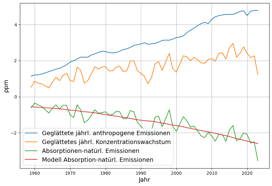
While the absorption constant and the linear relationship between absorption and concentration are physically very well founded and proven, the assumption of constant natural emissions appears arbitrary. Therefore, instead of a constant expression , it is enlightening to calculate the residual from the measured data and the calculated absorption constant instead
must be considered:
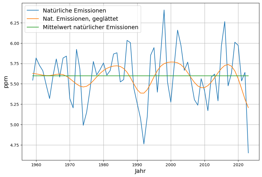
The mean value of results in the constant model term . A slight smoothing results in a periodic curve. Roy Spencer has attributed these fluctuations to the El Nino, although it is not clear whether the fluctuations are attributable to the absorptions or the natural emissions . But no long-term trend is discernible. Therefore, the question must be clarified as to why short-term temperature dependencies are present, but long-term global warming does not appear to have any correspondence in the model.
Temperature-dependent model
We now extend the model by additionally allowing a linear temperature dependence for both the absorptions and the other emissions . Since our measurement data only provide their difference, we can represent the temperature dependence of this difference in a single linear function of the temperature  , i.e.
  . Assuming that both and are temperature-dependent, the difference between the corresponding linear expressions is again a linear expression. Accordingly, the extended model has this form.
In principle, and  could be combined into a single constant. However, since depends on the temperature scale used, and on the unit of measurement of the CO2 concentration, we leave it at 2 constants.
CO2 concentration as a proxy for temperature
As already explained in the publication in section 2.3.2, there is a high correlation between CO2 concentration and temperature. Where this correlation comes from, i.e. whether there is a causal relationship (and in which direction) is irrelevant for this study. However, we are not establishing the correlation between  and
and  here, but between (temperature) and
  (CO2 concentration without logarithm).
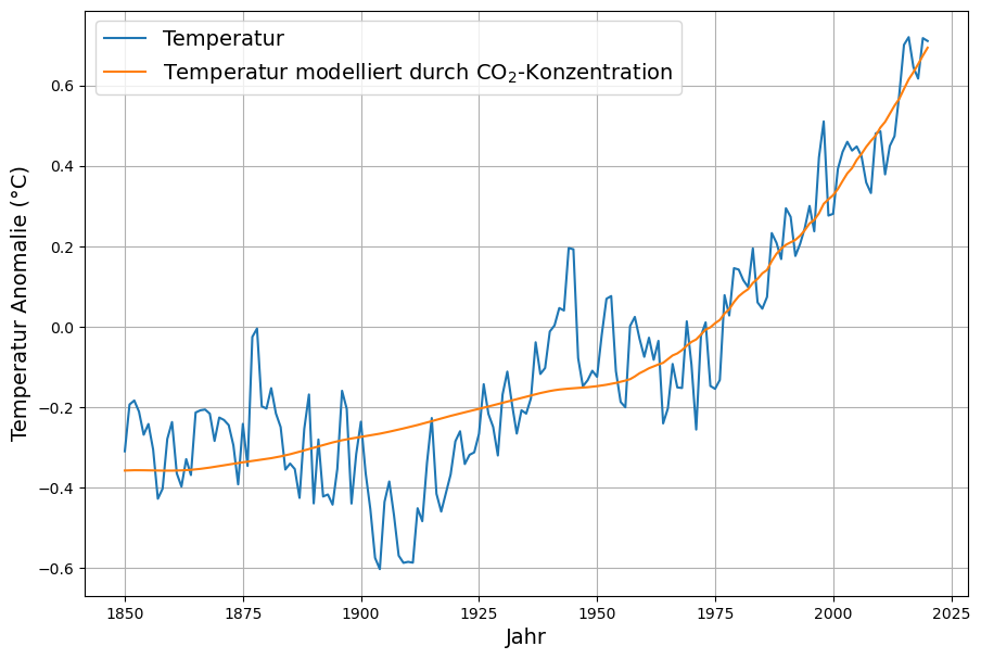
As a result, the temperature anomaly can be derived from the concentration using the linear function
with
can be approximated.
Use of the CO2 proxy in the temperature-dependent equation
If we now experimentally insert the proxy function for the temperature into the temperature-dependent equation, we obtain the following equation:
and
The expression on the right-hand side now has the same form as the original equation, i.e.
with

Conclusions
Therefore, with a linear dependence of temperature on CO2 concentration, temperature effects of sinks and sources cannot be distinguished from concentration effects, both are included in the “effective” absorption constant and the constant of natural emissions . Therefore, the simple source and sink model contains all linear temperature effects.
This explains the astonishing independence of the model from the global temperature increase of the last 50 years.
This correlation also suggests that the absorption behavior of atmospheric sinks will not change in the future.
However, if we want to know exactly how the temperature will affect the sources and sinks, other data sources must be used. This knowledge is not necessary for forecasting future CO2 concentrations from anthropogenic emissions due to the correlation found.