Temperature Dependent CO2 Sink model

In the simple model of CO₂ sinks and natural emissions published in this blog and elsewhere, the question repeatedly arose in the discussion: How is the — obvious — temperature dependence of natural CO₂ sources, for example the outgassing oceans, or sinks such as photosynthesis, taken into account?

The model shows no long-term temperature dependence trend, only a short-term cyclical dependence. A long-term trend in temperature dependence over the last 70 years is not discernible even after careful analysis.
In the primary publication, it was ruled out that the absorption coefficient could be temperature-dependent (Section 2.5.3). However, it remained unclear whether a direct temperature dependence of the sources or sinks is possible. We re-visit the sink model in order to find a way to consider temperature dependence adequately.

Original temperature-independent model

For setting up the equation for mass conservation of CO₂ in the atmosphere (see equations 1,2,3 of the publication), we split the total yearly emissions into anthropogenic emissions $E_i$ in year $i$ , and all other, predominantly natural emissions $N_i$ . For simplification, the — more unknown than known — land use caused emissions are included in the natural emissions.
The increase of CO₂ in the atmosphere is
$G_i = C_{i+1} - C_i$ ,
where $C_i$ is atmospheric CO₂ concentration at the beginning of year $i$ .
With absorptions $A_i$ the mass balance becomes:
$E_i - G_i = A_i - N_i$
The difference between the absorptions and the natural emissions was modeled linearly with a constant absorption coefficient $a^0$ expressing the proportionality with concentration $C_i$ and a constant $n^0$ for the annual natural emissions

(1) $\begin{equation*}E_i - G_i = a^0\cdot C_i - n^0\end{equation*}$

The estimated parameters are:
$a^0=0.0183$ ,
$n^0=5.2$ ppm

While the proportionality between absorption and concentration by means of an absorption constant $a^0$ is physically very well founded, the assumption of constant natural emissions appears arbitrary.
Effectively this assumed constant contains the sum of all emissions except the explicit anthropogenic ones and also all sinks that are balanced during the year.
Therefore it is enlightening to calculate the estimated natural emissions $\hat{N_i}$ from the measured data and the mass balance equation with the estimated absorption constant $a^0=0.0183$ :
$\hat{N_i} = G_i - E_i + a^0\cdot C_i$

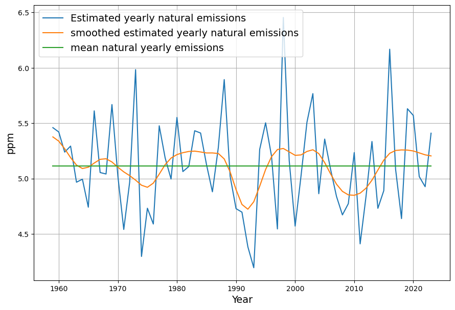
The mean value of $\hat{N_i}$ results in the constant model term $n^0$ . A slight smoothing results in a cyclic curve. Roy Spencer has attributed these fluctuations to El Nino. By definition a priori it cannot be said whether the fluctuations are attributable to the absorptions $A_i$ or to the natural emissions $N_i$ . In any case no long-term trend is seen.

The reconstruction $\hat{C_i}$ of the measured concentration data is done recursively from the model and the initial value taken from the original data:
$\hat{C_0} = C_0$
$\hat{C_{i+1}} = \hat{C_i} + E_i +n^0 - a^0\cdot \hat{C_i}$

Extending the model by Temperature

The sink model is now extended by a temperature term $T_i$ :

(2) $\begin{equation*}E_i - G_i = a\cdot C_i + b\cdot T_i + c\end{equation*}$

These 3 regression parameters can be estimated directly, but we do not know how the resulting numbers relate to the estimation without temperature dependence. Therefore we will motivate and build this model in an intuitive way.

The question arises why and how sources or sinks should be dependent on El Nino? It implies a temperature dependence. But why can’t the undeniable long term temperature trend be seen in the model? Why is there no trend in the estimated natural emissions?
The answer is in the fact that CO₂ concentration and temperature are highly correlated, at least since 1960, i.e. during the time when CO₂ concentration was measured with high quality:

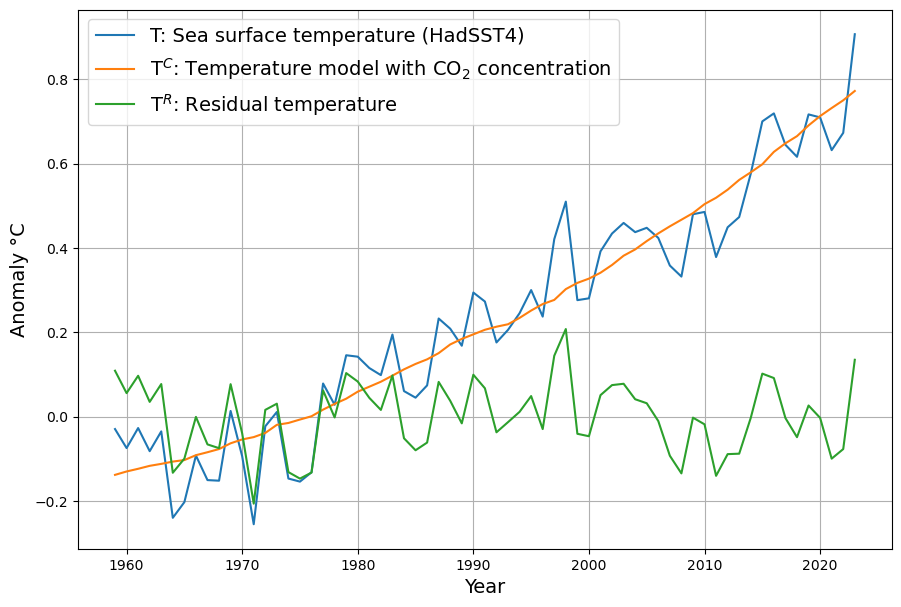
Therefore any longterm trend dependent on temperature would be attributed to CO₂ concentration when the model is based on concentration. This has been analysed in detail. We make no claim of causality between CO₂ concentration and temperature, in neither direction, but just recognise their strong correlation. The optimal linear CO₂ modelling for temperature anomaly based on the HadSST4 temperature data is:
$T_i^C = d\cdot C_i + e$
with $d=0.0082 \frac{^{\circ} C}{ppm}$ and $e = -2.7$ °C

The actual temperature $T_i$ is the sum of the modelled Temperature $T_i^C$ and the residual Temperature $T_i^R$
Therefore the new model equation becomes
$E_i - G_i = a\cdot C_i + b\cdot (T_i ^C + T_i^R)+ c$
Replacing $T_i^C$ with its CO2-concentration proxy
$E_i - G_i = a\cdot C_i + b\cdot (d\cdot C_i + e + T_i^R)+ c$
and re-arrangement leads to:
$E_i - G_i = (a + b\cdot d)\cdot C_i + b\cdot T_i^R+ (c + b\cdot e)$ .

Now the temperature part of the model depends only on zero mean variations, i.e. without trend.
All temperature trend information is covered by the coefficients of $C_i$ . This model corresponds to Roy Spencer’s observation that much of the cyclic variability is explained by El Nino, which is closely related to the “residual temperature” $T_i^R$ .
With $b=0$ we would have the temperature independent model above, and the coefficients of $C_i$ and the constant term correspond to the known estimated parameters. Due to the fact that $T_i^R$ does not contain any trend, the inclusion of the temperature dependent term does not change the other coefficients.

The estimated parameters of the last equation are:
$a + b\cdot d = 0.0183 = a^0$ ,
$b = -2.9\frac{ppm}{^{\circ}C}$ ,
$c + b\cdot e = -5.2 ppm = -n^0$ .

The first and last parameter correspond to those of the temperature independent model. But now, from the estimated $b$ coefficient, we now can evaluate the contribution of Temperature $T_i$ to the sinks and the natural emissions

The final determined parameters are
$a = a_0 - b\cdot d = 0.0436$ ,
$b = -0.29 \frac{ppm}{^{\circ}C}$ ,
$c = -n_0 - b\cdot e = -13.6ppm$

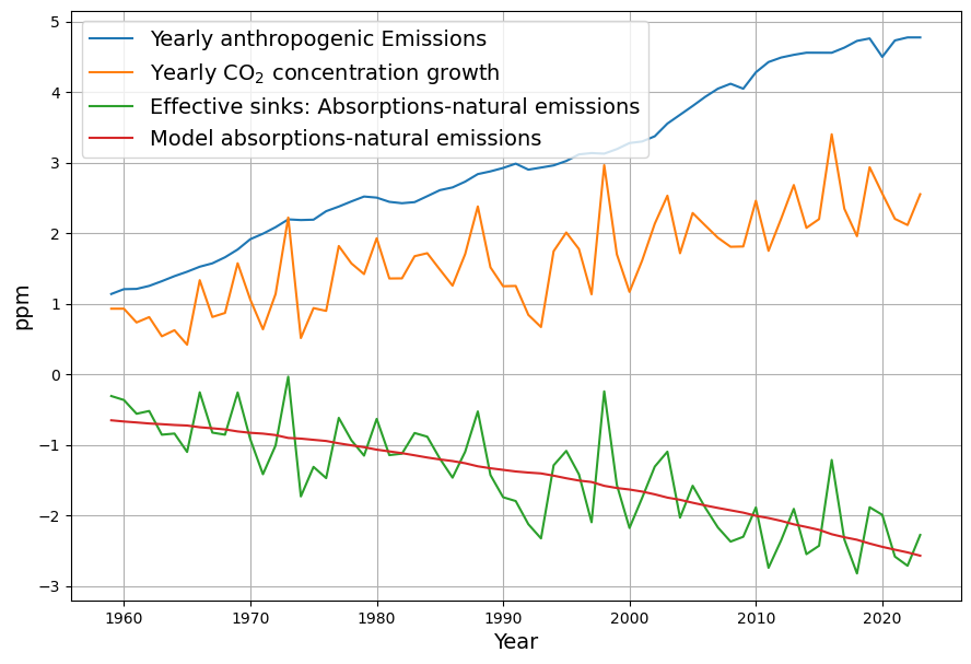
It is quite instructive how close the yearly variations of temperature matches the variations of the measured sinks:

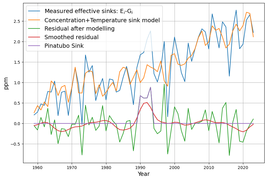
The smoothed residual is now mostly close to 0, with the exception of the Pinatubo eruption (after 1990) being the most dominant non-accounted signal after application of the model. Curiously in 2020 there is a reduced sink effect, most likely due to higher average temperature, effectively compensating the reduced emissions due to Covid lockdowns.
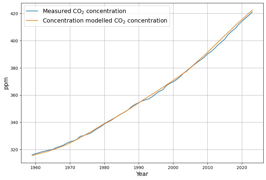
The model reconstruction of the concentration is now extended by the temperature term:
$\hat{C_0} = C_0$
$\hat{C_{i+1}} = \hat{C_i} + E_i - a\cdot \hat{C_i} - b\cdot T_i - c$

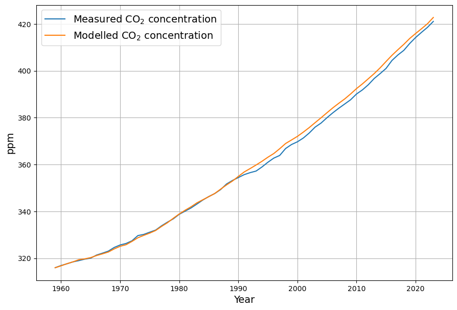
This is confirmed when looking at the reconstruction. The reconstruction only deviates at 1990 due to the missing sink contribution from the Pinatubo eruption, but follows the shape of the concentration curve precisely. This is an indication, that the Concentration+Temperature model is much better suited to model the CO2-concentration.
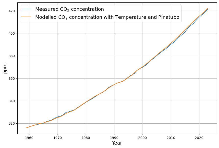
In order to compensate the deviations after 1990, the sink effect due to Pinatubo A $_i^P$ must be considered. It is introduced as a negative emission signal into the recursive modelling equation:
$\hat{C_{i+1}} = \hat{C_i} + E_i -A_i^P- a\cdot \hat{C_i} - b\cdot$
This reduces the deviations of the model from the measured concentration significantly:

Consequences of the temperature dependent model

The concentration dependent absorption parameter is in fact more than twice as large as the total absorption parameter, and increasing temperature increases natural emissions. As long as temperature is correlated to CO₂ concentration, the to trends cancel each other, and the effective sind coefficient appears invarant w.r.t. temperature.

The extended model becomes relevant, when temperature and CO₂ concentration diverge.

If temperature rises faster than according the above CO₂ proxy relation, then we can expect a reduced sink effect, while with temperatures below the expectancy value of the proxy the sink effect will increase.

As a first hint for further research we can estimate the temperature equilibrium concentration based on current measurements. This is given by (anthropogenic emissions and concentration growth at 0 by definition):
$a\cdot C + b\cdot T + c = 0$
$C = \frac{-b\cdot T - c}{a}$
For $T = 0°$ (= 14° C worldwide average temperature) we get as the – no emissions – equilibrium concentration.
$C = \frac{-c}{a} = \frac{-13.6}{0.0436} ppm = 312 ppm$

The temperature sensitivity is the Change of equilibrium concentration for 1° temperature change:
$\frac{\Delta C}{\Delta T} = \frac{-b}{a} = 66.5 \frac{ppm}{°C}$
Considering the fact the the temperature anomaly was appr. T = -0.5° in 1850, this corresponds very well with the assumed pre-industrial equilibrium concentration of 280 ppm.

A model for paleo climate?

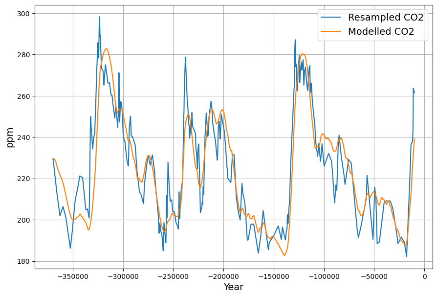
An important consequence of the temperature enhanced model is for understanding paleo climate, which is e.g. represented in the Vostok ice core data:

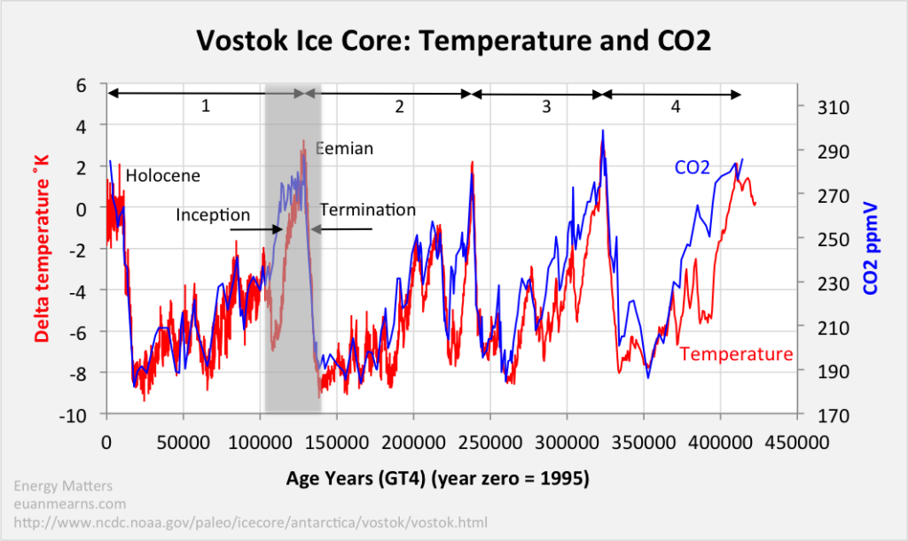
Without analysing the data in detail, with the temperature dependence of the CO₂ concentration we have a tool for e.g. estimating the equilibrium CO₂ concentration depending on temperature. Stating the obvious, it is clear that CO₂ concentration is controlled by temperature and not the other way round – the time lag between temperature changes and concentration changes is several centuries.

The Vostok data have been analysed with the same model of concentration and temperature dependent sinks and natural sources. Although the model parameters are substantially different due to the totally different time scale, the measured CO₂ concentration is nicely reproduced by the model, driven entirely by temperature changes: