How large is the Greenhouse Effect in Germany? — A statistical Analysis.

High correlation as an indication of causality?

The argument that CO₂ determines the mean global temperature is often illustrated or even justified with this diagram, which shows a strong correlation between CO₂ concentration and mean global temperature, here for example the mean annual concentration measured at Maona Loa and the annual global sea surface temperatures:

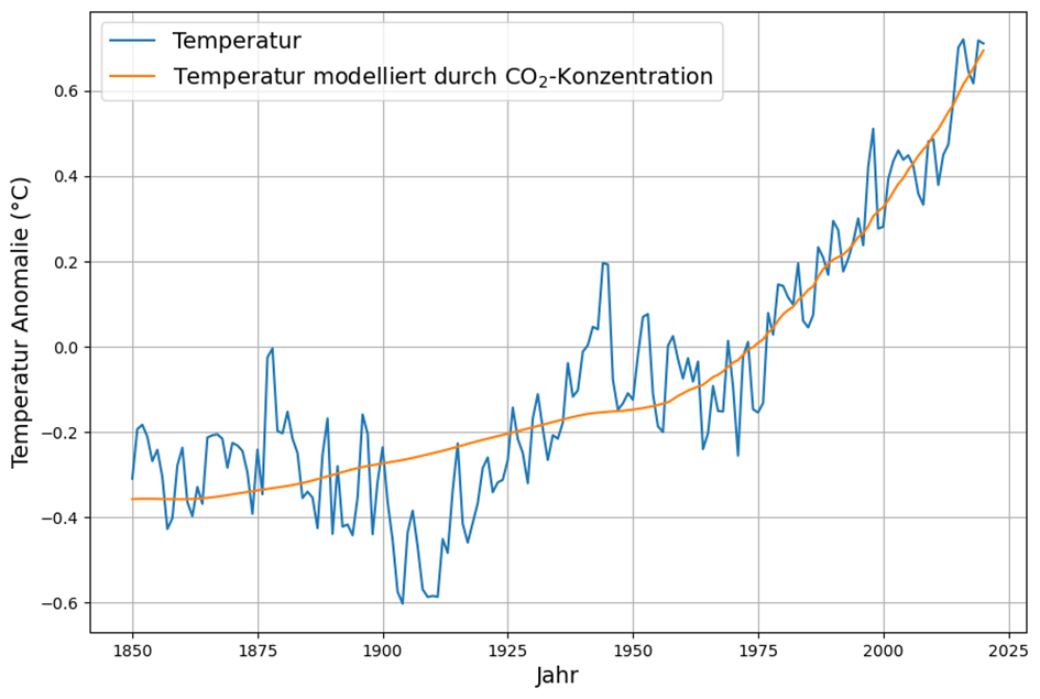
Although there are strong systematic deviations between 1900 and 1975 – 75 years after all – the correlation has been strong since 1975.
If we try to explain the German mean temperatures with the CO₂ concentration data from Maona Loa available since 1959, we get a clear description of the trend in temperature development, but no explanation of the strong fluctuations:

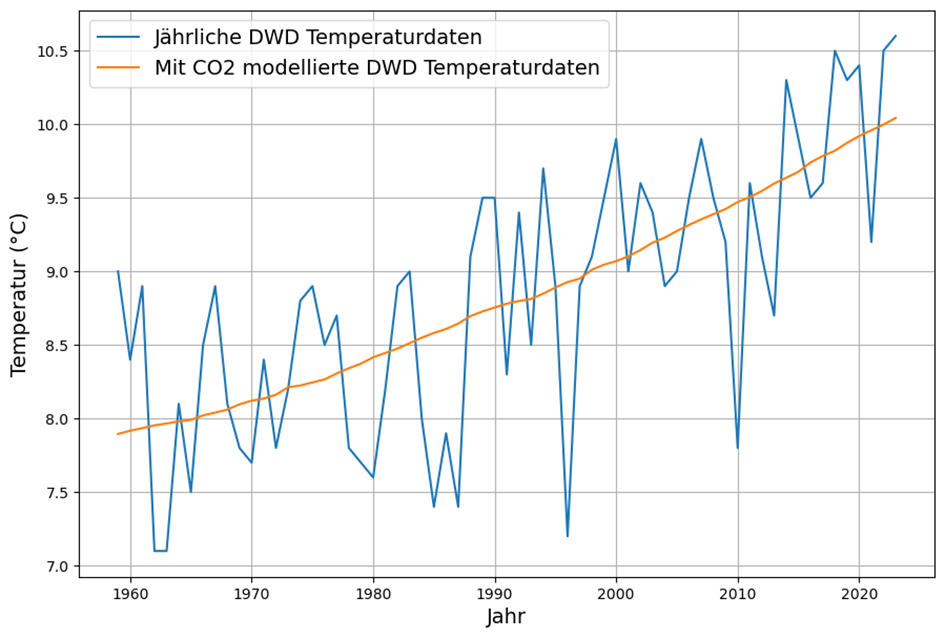
The “model temperature” estimated from the logarithmic CO₂ concentration data measured in year using the least squares method is given by
  (°C)

 If we add the annual hours of sunshine as a second explanatory variable, the fit improves somewhat, but we are still a long way from a complete explanation of the fluctuating temperatures. As expected, the trend is similarly well represented, and some of the fluctuations are also explained by the hours of sunshine, but not nearly as well as one would expect from a causal determinant:

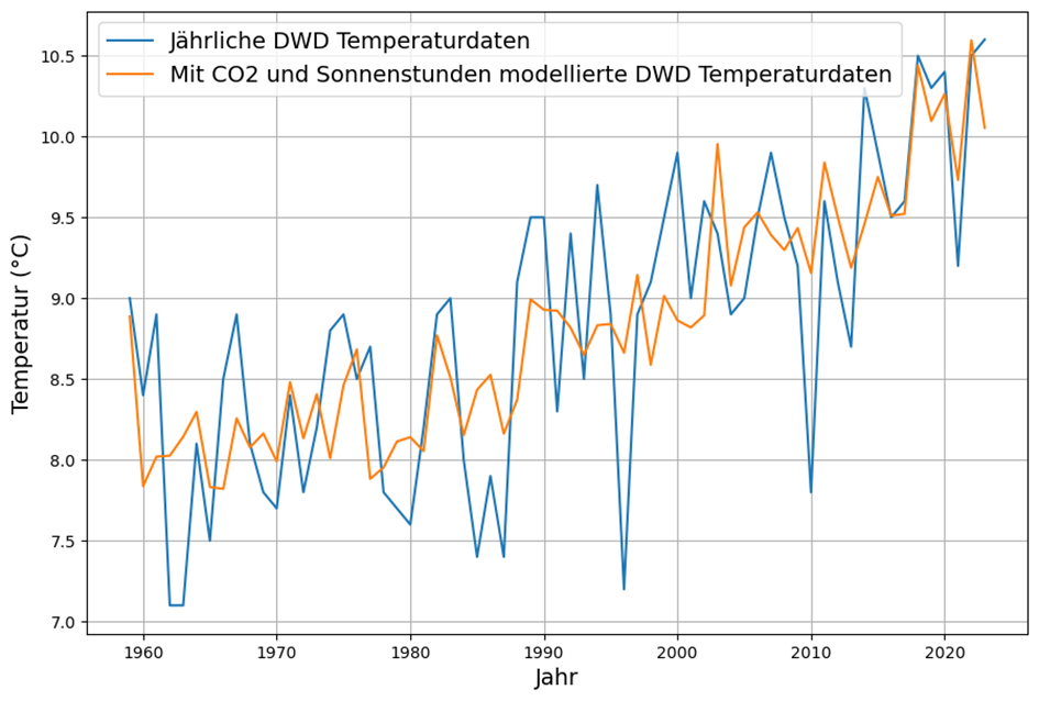
The model equation for the estimated temperature becomes with the extension of the hours of sunshine to
 (°C)
The relative weight of the CO₂ concentration has decreased slightly with an overall improvement in the statistical explanatory value of the data.

However, it looks as if the time interval of 1 year is far too long to correctly treat the effect of solar radiation on temperature. It is obvious that the seasonal variations are undoubtedly caused by solar radiation.
 The effects of irradiation are not all spontaneous; storage effects must also be taken into account. This corresponds to our perception that the heat storage of summer heat lasts for 1-3 months and that the warmest months, for example, are only after the period of greatest solar radiation. We therefore need to create a model based on the energy flow that is fed with monthly measured values and that provides for storage.

Energy conservation – improving the model

To improve understanding, we create a model with monthly data taking into account the physical processes (the months are counted with the index variable ):

• Solar radiation supplies energy to the earth’s surface, which is assumed to be proportional to the number of hours of sunshine per month ,

• assuming the greenhouse effect, energy is also supplied; a linear function of is assumed for the monthly energy input (or prevented energy output),
• the top layer of the earth’s surface stores the energy and releases it again; the monthly release is assumed to be a linear function of the surface temperature ,
• the monthly temperature change in Germany is assumed to be proportional to the energy change.

This results in this modeled balance equation, the constant makes it possible to use arbitrary measurement units:

On the left-hand side of the equation is the temperature change as a representative of the energy balance change, while the right-hand side represents the sum of the causes of this energy change.
To determine the coefficients using the least squares method, the measured temperature is used instead of the modeled temperature .

Here are the monthly temperature and sunshine hour data. It can be seen that the temperature data lags behind the sunshine hours data by around 1-2 months, but has a similar overall trend:

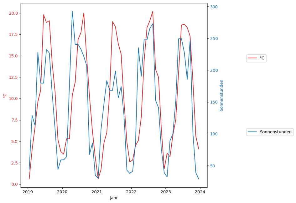
This fits with the assumption that we actually have a storage effect. The balance equation should therefore provide meaningful values. However, we need to take a closer look to evaluate the estimated result.

In this diagram, the values of the respective coefficients are shown in the first column, their standard error in the second column, followed by the so-called T-statistic, followed by the probability that the assumption of the coefficient other than 0 is incorrect, the so-called probability of error. This means that a coefficient is only significant if this probability is close to 0. This is the case if the T-statistic is greater than 3 or less than -3. Finally, the last two columns describe the so-called 95% confidence interval. This means that there is a 95% probability that the actual estimated value is within this interval.

     Coefficient  Std.Error   t-Value    P>|t|    [0.025     0.975]
--------------------------------------------------------------------
a       -0.4826     0.0142   -33.9049   0.0000    -0.5105   -0.4546
b        0.0492     0.0013    38.8127   0.0000     0.0467    0.0517
c        0.6857     0.9038     0.7587   0.4483    -1.0885    2.4598
d       -6.3719     5.3013    -1.2020   0.2297   -16.7782    4.0344

Here, the error probabilities of the coefficients and are so high, at 45% and 23% respectively, that we must conclude that both and also . measures the significance of the CO₂ concentration for the temperature. This means that the CO₂ concentration has had no statistically significant influence on temperature development in Germany for 64 years. However, this is the period of the largest anthropogenic emissions in history.
The fact that also assumes the value 0 is more due to chance, as this constant depends on the units of measurement of the CO₂ concentration and the temperature.

As a result, the balance equation is adjusted:

 with the result:

       Coefficient  Std.Error   t-Value    P>|t|    [0.025    0.975]
--------------------------------------------------------------------
a         -0.4823     0.0142   -33.9056   0.0000   -0.5102   -0.4544
b          0.0493     0.0013    38.9661   0.0000    0.0468    0.0517
d         -2.3520     0.1659   -14.1788   0.0000   -2.6776   -2.0264

The constant is now valid again with high significance due to the fact that . The other two coefficients and have hardly changed. They deserve a brief discussion:

The coefficient indicates which part of the energy measured as temperature is released again over the course of a month. This is almost half. This factor is independent of the zero point of the temperature scale; choosing K or anomalies instead of °C would result in the same value. The value corresponds approximately to the subjective perception of how the times of maximum temperature in summer shift in time compared to the maximum solar radiation.
The coefficient indicates the factor by which the hours of sunshine translate into monthly temperature changes.

The result is not just an abstract statistic, it can also be visualized by reconstructing the monthly temperature curve of the last 64 years with the help of the model described.

The reconstruction of the entire temperature curve is based on the time series of sunshine hours and a single temperature starting value , the temperature of the month preceding the beginning of the time series under investigation since 1959, in this case December 1958.
The reconstruction is carried out using this recursion from the sunshine hours over the 768 months from January 1959 to December 2023:

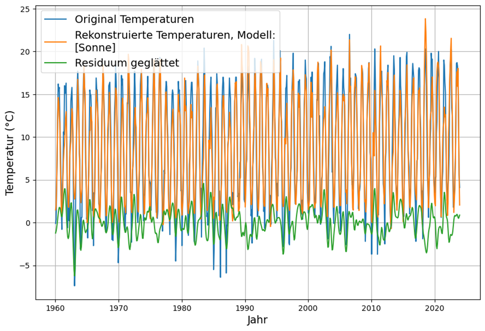
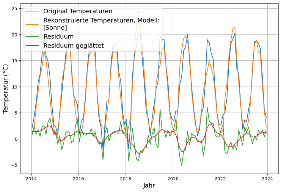
Here is the complete reconstruction of the temperature data in comparison with the original temperature data:

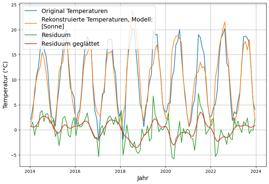
 The last 10 years are shown enlarged for a clearer presentation:

It is noticeable that the residual, i.e. the deviations of the reconstruction from the actual temperatures up to the end of the investigated period around 0, appears symmetrical and shows no obvious systematic deviations. The measure of the error of the reconstruction is the standard deviation of the residual. This is 2.5°C. Since we are investigating a long period of 64 years, a fine analysis of the long-term trends of original temperatures, reconstruction and residual could find a possible upper limit of the possible influence of CO₂

Detailed analysis of the residue

If we determine the average slope of the three curves – original temperature data, reconstruction and residual – over the entire 64-year period by estimating an equalization line, we obtain the following long-term values:

• Original temperature data: 0.0027 °C/month = 0.032 °C/year
• Reconstructed temperature data: 0.0024°C/month = 0.029 °C/year
• Residual: 0.00028 °C/month = 0.0034 °C/year

Of the original temperature trend, 90% is explained by the number of hours of sunshine. This leaves only 10% of unexplained variability for other causes. Until proven otherwise, we can therefore assume that the increase in CO₂ concentration is responsible for at most these 10%, i.e. for a maximum of 0.03° C per decade over the last 64 years. Statistically, however, the contribution of the CO₂ concentration cannot be considered significant. It
should be borne in mind that this simple model does not take into account many influencing factors and inhomogeneities, meaning that the influence of the CO₂ concentration is not the only factor that is effective in addition to the hours of sunshine. This is why the CO₂ influence is not considered statistically significant.

Extension – correction by approximation of the actual irradiation

So far, we have used the hours of sunshine as a representative of the actual energy flow. This is not entirely correct, because an hour of sunshine in winter means significantly less irradiated energy than in summer due to the much shallower angle of incidence.

The seasonal course of the weighting of the incoming energy flow has this form. The hours of sunshine must be multiplied by this weighting to obtain the energy flow.

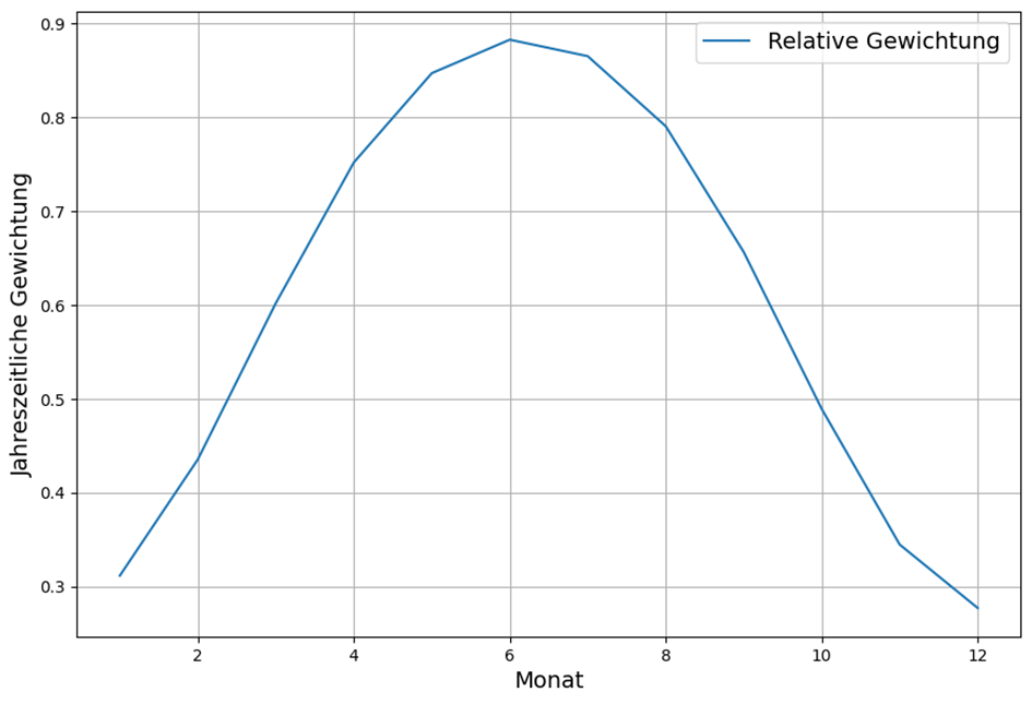
With these monthly weightings, the model is again determined from solar radiation and CO2. Again, the contribution of CO2 must be rejected due to lack of significance. Therefore, the reconstruction of the temperature from the irradiating energy flow is slightly better than the above reconstruction.

The standard deviation of the residual has been reduced to 2.1°C by correcting the hours of sunshine to the energy flow.

Possible generalization

Worldwide, the recording of sunshine hours is far less complete than that of temperature measurements. Therefore, the results for Germany cannot simply be reproduced worldwide.
 However, satellites are used to measure cloud cover and the reflection of solar radiation on clouds. This data leads to similar results, namely that the increase in CO₂ concentration is responsible for at most 20% of the global average temperature increase. As this is lower on average than the temperature increase in Germany, this also ultimately leads to an upper limit of 0.03°C per decade for the consequences of the CO₂ -induced greenhouse effect.