The Extended Carbon Sink Model (work in progress)

Introduction – potential deficit of the simple linear carbon sink model

With the simple linear carbon sink model the past relation between anthropogenic emissions and atmospheric CO2 concentration can be excellently modelled, in particular when using the high quality emission and concentration data after 1950.
The model makes use of the mass conservation applied to the CO2-data, where is the CO2 concentration in year , are the anthropogenic emissions during year , are all other CO2 emissions during year (mostly natural emissions), and are all absorptions during year . We assume emissions caused by land use change to be part of the natural emissions, which means that they are assumed to be constant. Due to the fact that their measurement error is very large, this should be an acceptable assumption.
With the concentration growth

we get from mass conservation the yearly balance

and are measured from known data sets (IEA and Maona Loa), and we define the effective sink as

The atmospheric carbon balance therefore is

The effective sink ist modelled as a linear function of the CO2-concentration by minimizing

w.r.t. and , where

The equation can be re-written to

where

is the average reference concentration represented by the oceans and the biosphere. The sink effect is proportional to the difference of the atmospheric concentration and this reference concentration. In the simple linear model the reference concentration is assumed to be constant, implying that these reservoirs are close to inifinite. Up to now this is supported by the empirical data.
This procedure is visualized here:

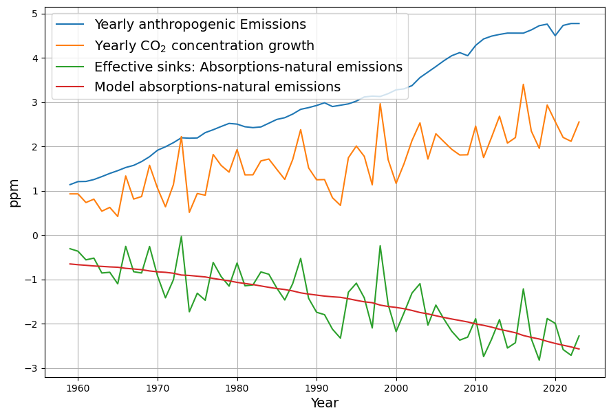
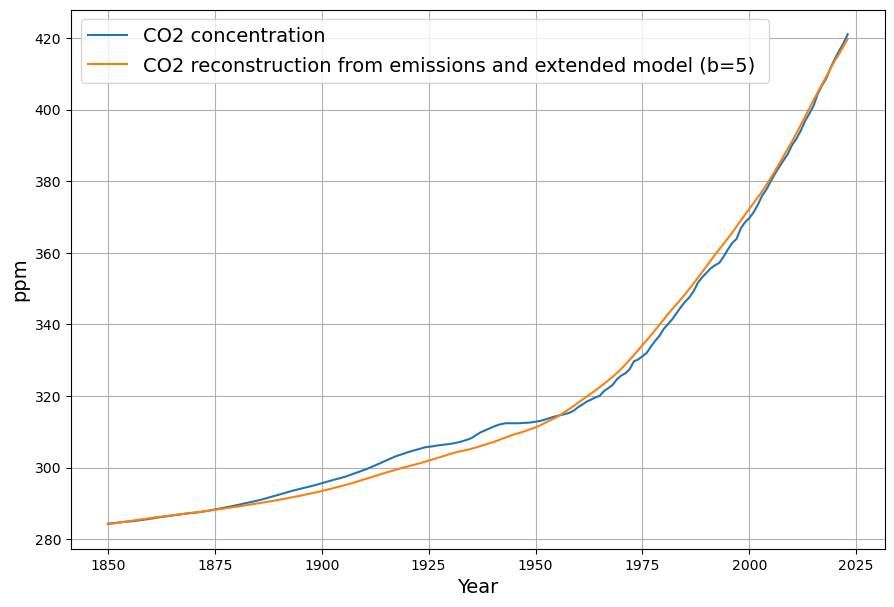
This results in an excellent model reconstruction of the measured concentration data:

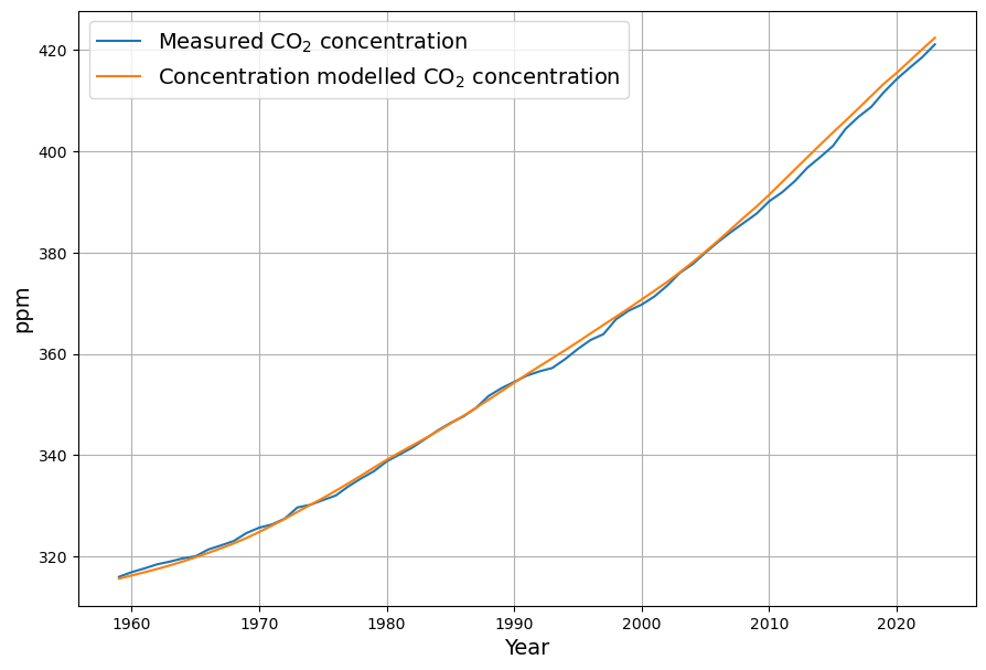
It is important to note that the small error since 2010 is an over-estimation of the actual measured data, which means that the estimated sink effect is under-estimated. Therefore we can safely say that currently we do not see the slightest trend of a possible decline of the 2 large sink systems, the ocean sink and the land sink from photosynthesis.

Nevertheless it can be argued that in the future both sink systems may enter a state of saturation, i.e. a lack of the ability to absorb surplus carbon from the atmosphere. As a matter of fact it is claimed from the architects of the Bern model and representatives of the IPCC that the capacity of the ocean is not larger than 5 times the capacity of the atmosphere, and therefore future ability to take up extra CO2 will rapidly decline. We don’t see this claim justified by data, but before we can prove that the claim is not justified, we will adapt the model to make it capable of calculating varying sink capacities.

Extending the model with a second finite accumulating box

In order to take care of the finite size of both the ocean and the land sinks, we do not pretend that these sink systems are infinite, but assume a second box besides the atmosphere with a concentration , taking up all CO₂ from both sink systems. The box is assumed to be times larger than the atmosphere, therefore for a given sink-related change of atmosphere concentration () we get an increase of concentration in the “sink box” of the same amount () but reduced by the factor b:

The important model assumption is that is the reference concentration, which determines future sink ability.
The initial value is the previously calculated equilibrium concentration

Therefore by evaluation of the recursion we get

The main modelling equation is adapted to

or

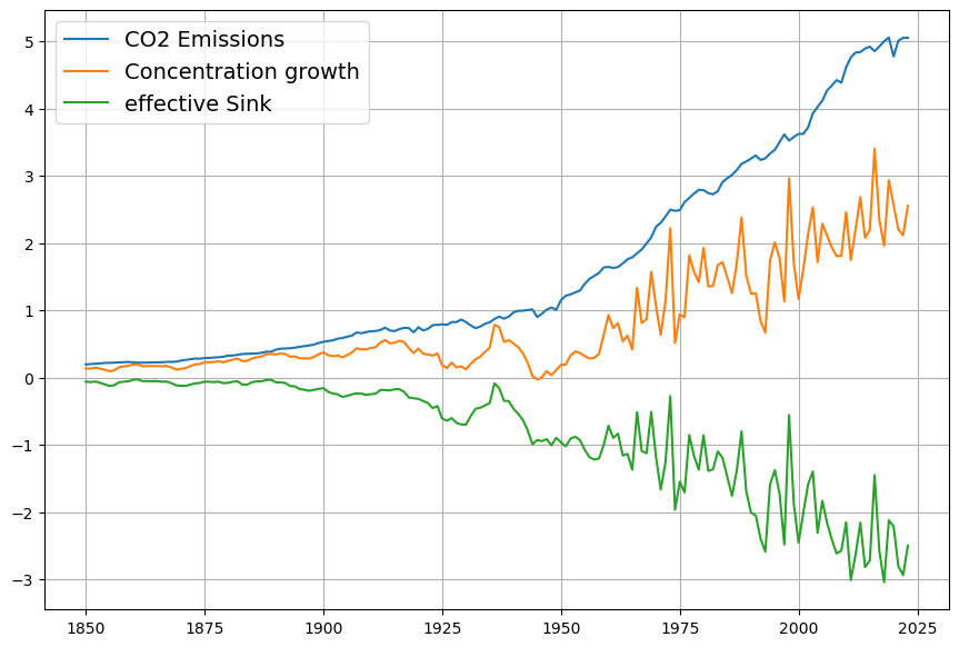
Obviously measurements must be started at the time where the anthropogenic emissions are still close to 0. Therefore we begin with the measurements from 1850, being aware that the data before 1959 are much less reliable than since then. There are reasons to assume that before 1950 land use change induced emissions play a stronger role than later. But there are strong reasons, that the estimated IEA values are too large, so in order to reach a reference value close to 280 ppm, an aequate weight for land use change emissions is 0.5.

Results for different scenarios

We will now evaluate the actual emission and concentration measurements for 3 different scenarios, for b=5, b=10, and b=50.
The first scenario (b=5) is considered to be the worst case scenario, rendering similar results as the Bern model.
The last scenario (b=50) corresponds to the “naive” view that the CO2 in the oceans is equally distributed, making use of the full potential buffer capacity of the oceans.
The second scenario (b=10) is somewhere in between.

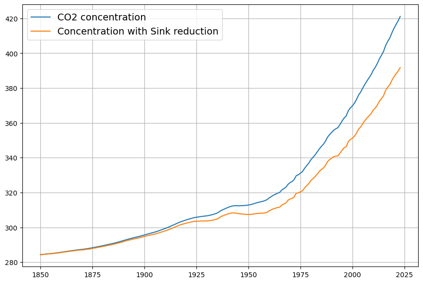
Szenario b=5: Oceans and land sinks have 5 times the atmospheric capacity

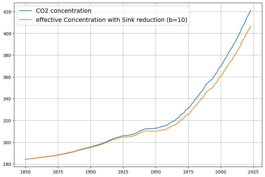
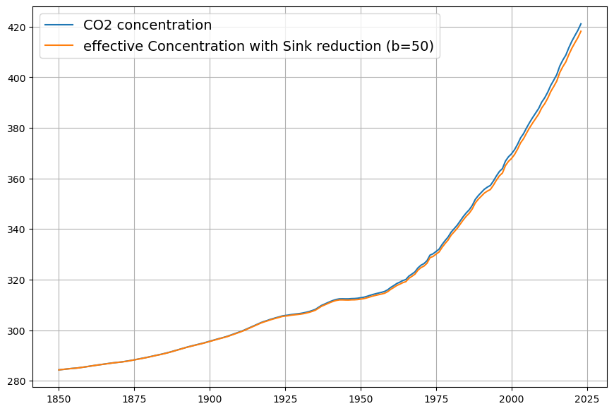
The “effective Concentration” used for estimating the model reduces the measured concentration by the weighted cumulative sum of the the effective sinks with . We see, that before 1900 there is hardly any difference to the measured concentration:

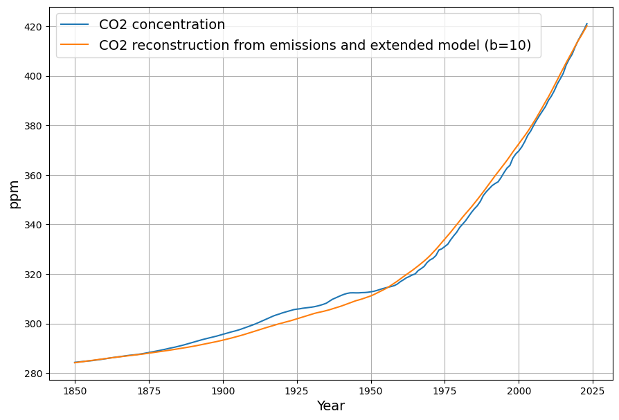
First we reconstruct the original data from the model estimation:

Now we calculate the future scenarios:

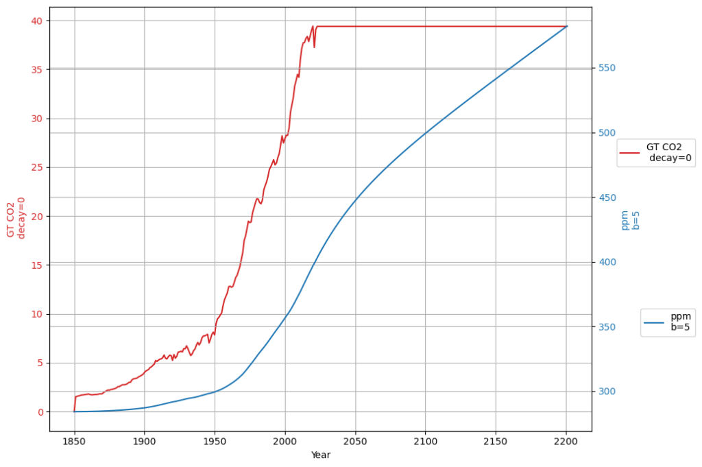
Constant emissions after 2023

In order to understand the reduced sink factor, we first investigate the case where emissions remain constant after 2023. By the end of 2200 CO2 concentration would be close to 600 ppm, with no tendency to flatten.

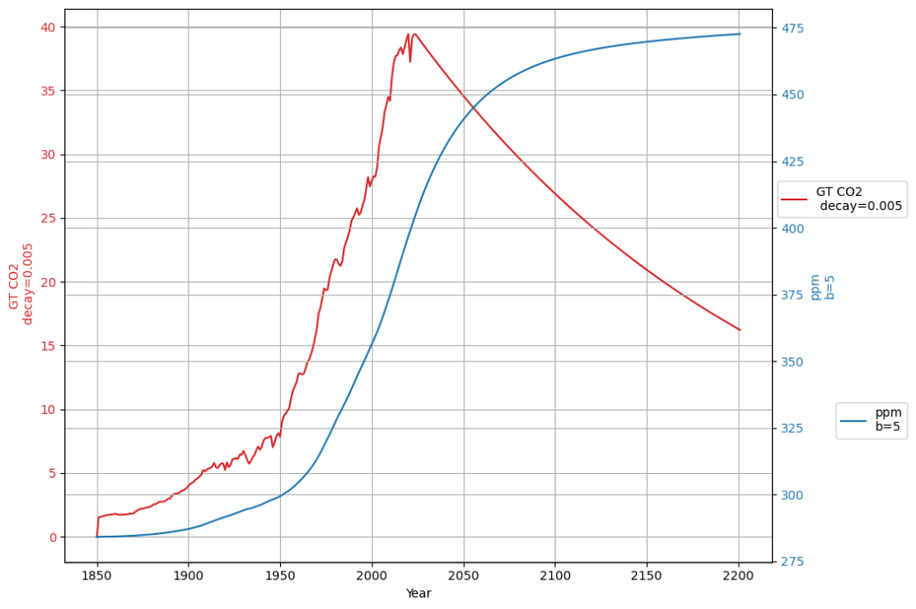
Emission reductions to reach equilibrium and keep permanently constant concentration

It is easy to see that under the given conditions of a small CO₂ buffer, the concentration keeps increasing when emissions are constant. The interesting question is, how the emission rate has to be reduces in order to reach a constant concentration.
From the model setup one would assume that the yearly emission reduction should be , and indeed, with a yearly emission reduction of 0.5% after 2023, we reach a constant concentration eventually and hold it. This means that emission rates have to be cut to half within 140 years – provided the pessimistic assumption turns out to be correct:

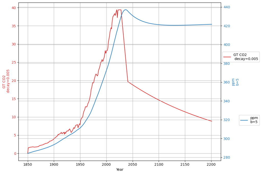
Fast reduction to 50% emissions, then keeping concentration constant

An interesting scenario is the one, which cuts emissions to half the current amout within a short time, and then trying to keep the concentration close to the current level:

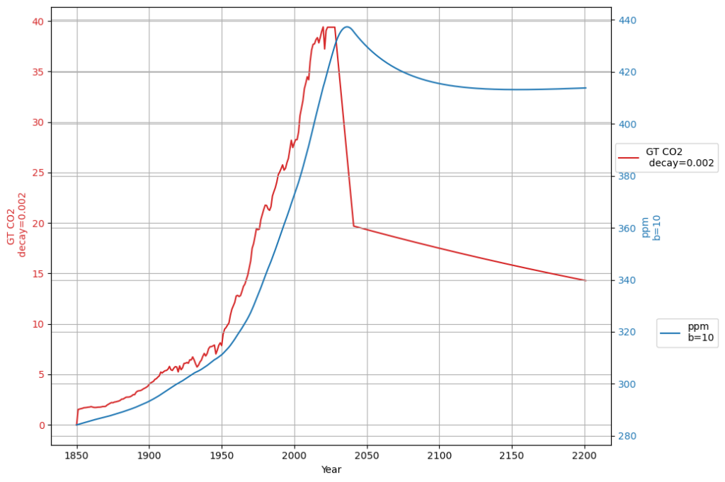
Scenario b=10: Oceans and land sinks have 10 times atmospheric capacity

Assuming the capacity of the (ocean and plant) CO2 reservoir to be 10-fold results, as expected, to half the sink reduction.

It does not change significantly the model approximation quality to the actual CO2 concentration data:

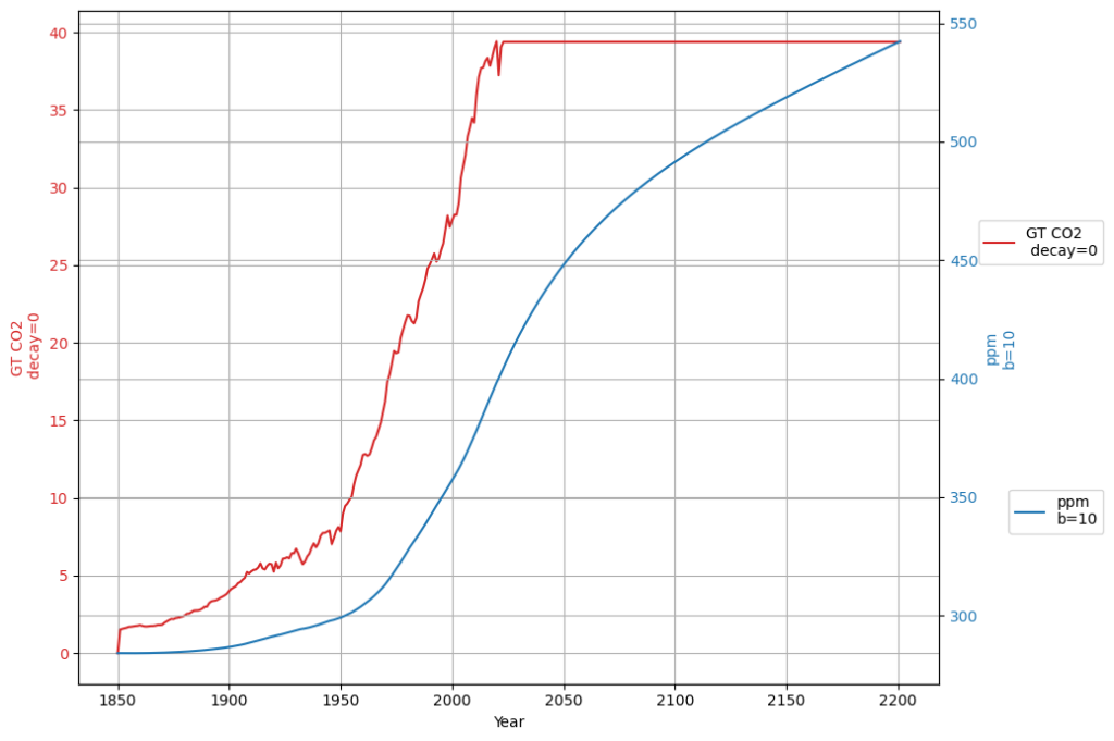
Constant emissions after 2023

The growth of the concentration for constant emissions is now smaller than 550 ppm by the end of 2200, but still growing.

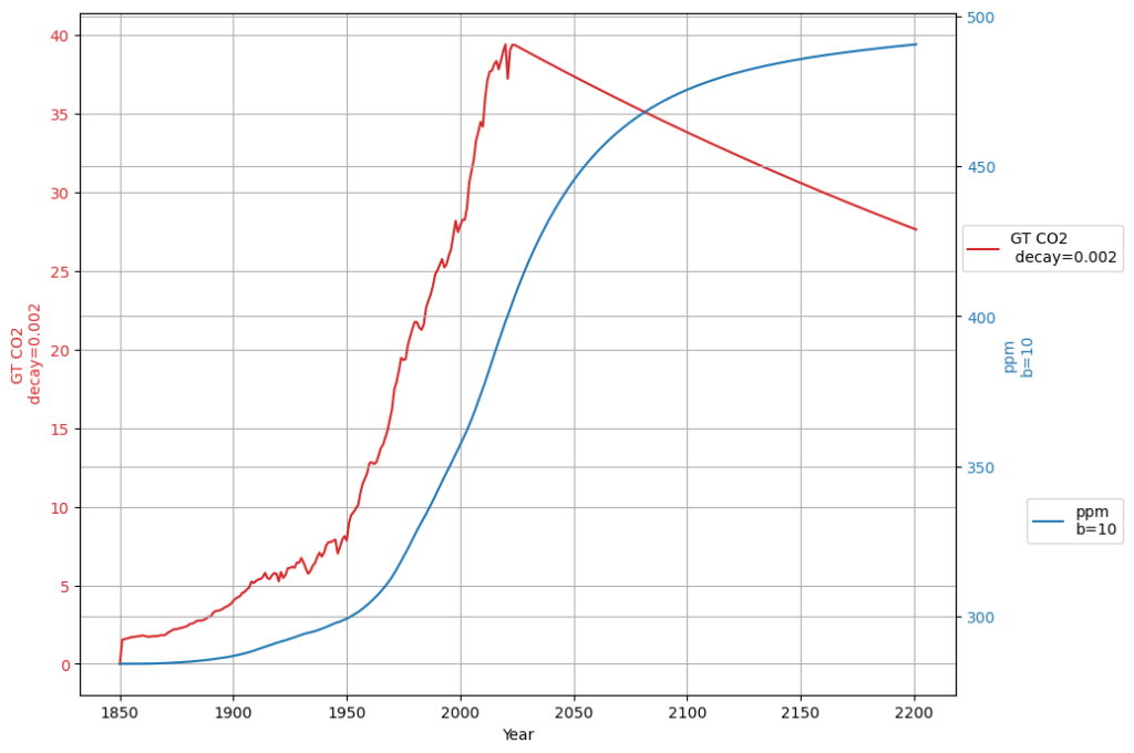
Emission reductions to reach equilibrium and keep permanently constant concentration

The emission reduction rate can be reduced to 0.2% in order to compensate the sink reduction rate:

Fast reduction to 50% emissions, then keeping concentration constant

This is easier to see for the scenario, which reduces swiftly emissions to 50%. with peak concentration below 440 ppm, the further slow reduction with 0.2% p.a. keeps the concentration at about 415 ppm.

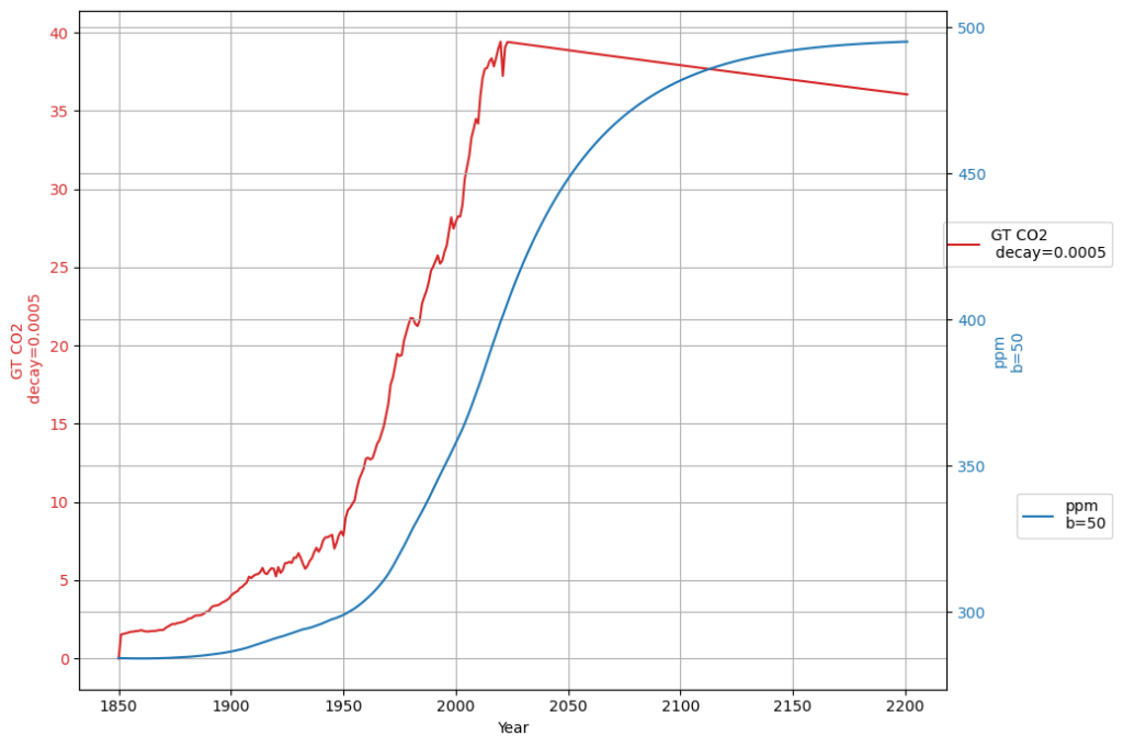
Szenario b=50: Oceans and land sinks have 50 times the atmospheric capacity

This scenario comes close to the original linear concentration model, which does not consider finite sink capacity.

Again, the reconstruction of the existing data shows no large deviation:

Constant emissions after 2023

Emission reductions to reach equilibrium and keep permanently constant concentration

We only need a yearly reduction of 0.05% for reaching a permanently constant CO2 concentration of under 500 ppm:

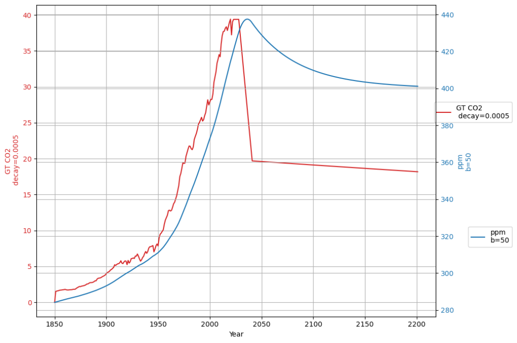
Fast reduction to 50% emissions, then keeping concentration constant

This scenario hardly increases today’s CO2-concentration and approximates eventually 400 ppm:

How to decide which model parameter b is correct?

It appears that with measurement data up to now it cannot be decided whether the sink receivers are finite, and if so, how limited they are.

The most sensitive detector from simple non-disputed measurements appears to be the concentration growth. I can be measured from both the actually measured data in the past,

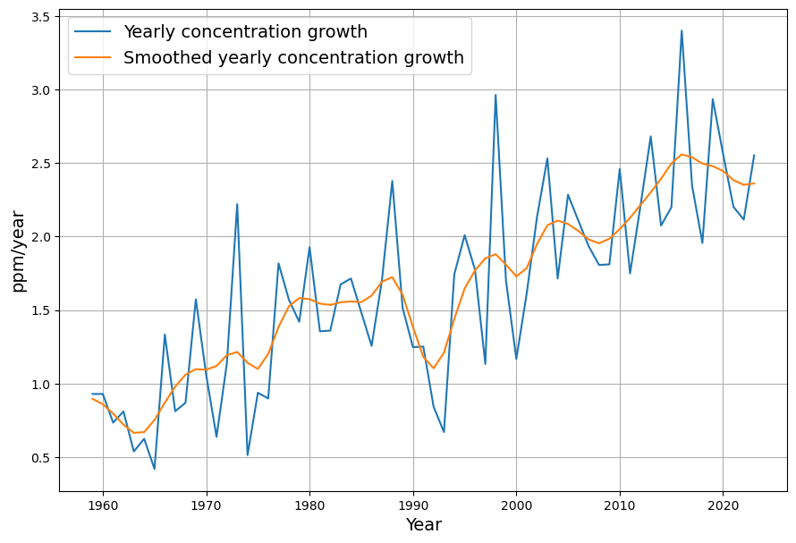
but also in the modelled data at any time. When comparing the concentration growth with future constant emissions of the 2 cases b=5 and b=50, we get this result:

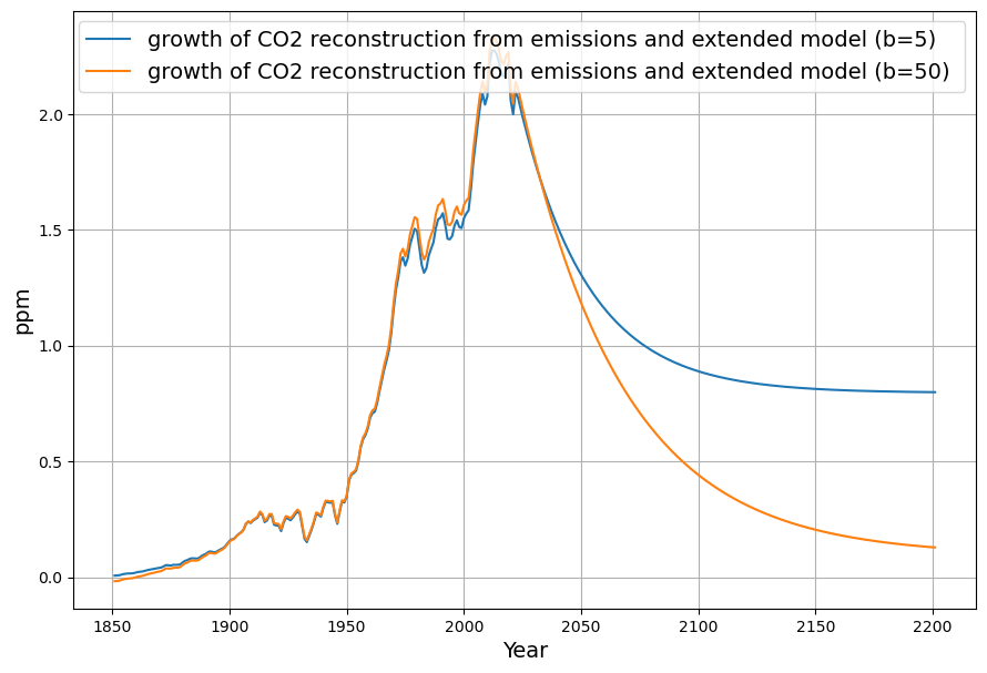
This implies that with the model b=5 concentration growth will never be under 0.8 ppm, whereas with the model b=50 the concentration growth decreases to appr. 0.1 ppm. But these large differences will only show up in many years, apparently not before 2050.

Preliminary Conclusions

Due to the fact that measurement data up to the current time can be reproduced well by both the Bern model as well as the simple linear sink model, it cannot be reliably decided with current data yet how large the effective size of the carbon sinks are. When emissions remain constant for a longer period of time, we expect to be able to perform a statistical test for the most likely value of the sink size factor b.

Nevertheless this extended sink model allows us to calculate the optimal rate of emission reduction for a given model assumption. Even in the worst case the required emission reduction is so small, so that any short term “zero emission” targets are not justified.

A related conclusion is the possibility of a re-calculation of the available CO₂-budget. Given a target concentration C the total bugdet is the amount of CO₂ required to fill up both atmosphere and accumulating box up to the target concentration.
Obviously the target concentration must be chosen in such a way, that it is compatible with the environmental requirements.