Do the carbon sinks fail? Or rather their models?

Introduction – the model dilemma

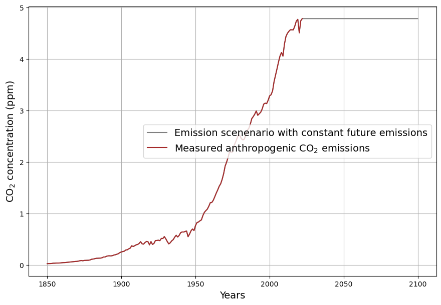
There is broad consensus that the increase in atmospheric CO₂ concentrations since 1850 is due to the sharp rise in anthropogenic CO₂ emissions since that time. Anthropogenic emissions have remained constant within the margin of measurement accuracy for around 10 years, and no major deviation from this trend is expected in the future. For illustrative purposes, constant emissions are assumed for the future scenario, based on the IEA’s Stated Policy Scenario. This debatable assumption is irrelevant for the actual calculation, as it is based exclusively on measurements of past data. The measured emissions and the assumed future emissions scenario are shown in Fig. 1. The use of the somewhat unusual unit of measurement ppm for emissions is due to the need to compare emissions and concentration ((1 ppm = 2.123 Gt C = 7.8 Gt CO₂).

Fig. 1: Measured anthropogenic emissions (brown), scenario of future constant emissions (grey)

Anthropogenic emissions do not remain entirely in the atmosphere. Their concentration has so far grown only about half as fast as it would have if all anthropogenic emissions had remained in the atmosphere, as shown in Fig. 2. This correlation has been valid since around 1950, when the phase of strongest emission growth of about 4% per year began, which continued until the mid-1970s.

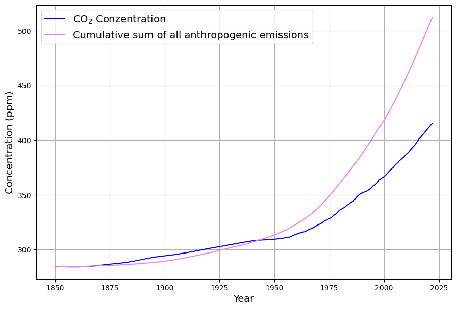
Fig. 2: Curve of actual CO2-concentration in the atmosphere (blue), hypothetical curve, if all emissions had remained in the atmosphere (purple).

The somewhat strange circumstance that between 1875 and 1945 the actual concentration is greater than the hypothetical concentration, in which all anthropogenic emissions remain in the atmosphere, is probably due to the fact that the significantly high emissions in the first half of the 20th century due to land use changes were not taken into account here. This also plays only a very limited role in the calculations made here, because only data after 1960 is used to calculate the result.

The reduced increase in concentration compared to anthropogenic emissions is due to the two major sink systems, land plants and the world’s oceans, both of which absorb considerable amounts of CO₂. The important question is what this absorption depends on, and more importantly, how the strength of absorption will develop in the future. This is reflected in the various sink models. Of the many variations of these models, two important, fundamentally different representatives are currently being investigated:

the linear sink model, in which the sink effect is a strictly linear function of CO2 concentration,
the Bern model, which assumes that about 20% of emissions remain in the atmosphere for a very long time.

Which of the models is correct has serious implications for how we deal with CO2. If some of it remains in the atmosphere virtually forever, this ultimately implies the need to reduce anthropogenic emissions to zero, i.e., budgeting, which is currently the political goal in Germany and the EU. If, on the other hand, the linear model is correct, we could rely on the fact that as concentrations rise, more CO₂ will be absorbed and the Paris climate target of balancing CO2 sources and sinks will be achieved in the second half of this century, even if emission patterns remain largely unchanged.

This article therefore focuses on finding a criterion to prove the correctness of one or the other model using existing measurement data.

What are sinks? A formal description

First, the measurable sink effect $S_i$ of year $i$ is determined as a result of the conservation of the total atmospheric mass of CO₂ using the continuity equation. The increase in concentration $G_i$ in the atmosphere is calculated as the difference between all emissions, i.e., anthropogenic emissions $E_i$ and natural emissions $N_i$ , and total absorption $A_i$ :

$G_i= C_i - C_{i-1} = E_i + N_i - A_i$ (Equation 1)

The global sink effect $S_i$ is the part of anthropogenic emissions $E_i$ that does not contribute to the increase in concentration $G_i$ :

$S_i = E_i - G_i$ (Equation 2)

This sink effect can be determined from the available emission and CO₂ concentration data (monthly concentration data from Mauna Loa) without modeling and is shown in Figure 3 as a time series from 1960 onwards. The data on the monthly measured concentration increase are seasonally adjusted by determining the difference from the same month of the previous year. Emissions and concentration are measured in the same unit of measurement ppm (1 ppm = 2.123 Gt C = 7.8 Gt CO₂).

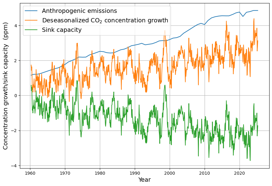
Fig. 3: Monthly emission data (blue), monthly concentration growth (orange), and monthly sink effect (green). The sink effect is drawn with negative sign, in order to separate it from the concentration growth in the graph.

Consequently, the sink effect is also the difference between absorptions $A_i$ and natural emissions $N_i$

$S_i = A_i -N_i$ (Equation 3)

It also follows that emissions from land use changes, which are subject to considerable uncertainty, are calculated as belonging to the unknown natural emissions.

The global sink effect defined in this way can be easily measured. Therefore, a method is sought to evaluate the respective sink model using the measured sink effect. The aim of this study is not to evaluate the correctness of the respective models based on their assumed causal mechanisms, but solely to find a mathematical statistical criterion for deciding, on the basis of measurement data, which model better corresponds to reality¹.

The two sink models

The linear sink model

Two sink models are compared. One, the “linear sink model” or “bathtub model,” assumes that the sink effect in year $i$ , $S_i$ , increases strictly linearly with the CO₂ concentration (of the previous year) $C_{i-1}$ (a more detailed analysis shows that the expected value of the time difference between concentration and sink effect is approximately 15-18 months):

$S_i = a\cdot C_{i-1} + b = a\cdot(C_{i-1} - C^0)$ (Equation 4)

where $C^0=-b/a$ represents the assumed pre-industrial equilibrium concentration without anthropogenic emissions.

The data for the period 1960-2025 yield the following estimates:

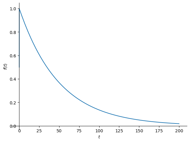
$a=0.0174, b=-4.87, C^0 =280 ppm   The estimated equilibrium concentration$ C^0 $corresponds remarkably well with the commonly assumed pre-industrial concentration of 280 ppm.   The model equation is a first-order differential equation with the impulse response  $ IRF^{linear}(t)=e^{-\frac{t}{\tau}} $  with$ \tau=1/a\approx 57 $years.   The crucial point is that the impulse response decays completely to 0, which means that atmospheric CO₂ is completely absorbed by the sinks over time.   <figure class="wp-block-image size-full is-resized"><img src="https://klima-fakten.net/wp-content/uploads/2025/10/Unbenannt.png" alt="" class="wp-image-12078" style="width:927px;height:auto"/><figcaption class="wp-element-caption">Fig. 4: Linear sink model, impuls response function (IRF) of the atmospheric concentration, time constant 57 years</figcaption></figure>   <h5 class="wp-block-heading">The Bern Model</h5>   In order to avoid drawing premature conclusions from the Bern model, it seems important to first consider a precursor to the Bern model, the so-called 2-box model. The starting point for the 2-box model is <strong>the fundamentally correct assumption that CO₂ sinks, the oceans and land plants, are finite and can only absorb a limited amount of CO₂</strong>. The simplest model that takes this fact into account is the 2-box model shown in Fig. 5, in which the atmosphere represents one box and the oceans together with land plants represent the second box.   <figure class="wp-block-image size-full"><img src="https://klima-fakten.net/wp-content/uploads/2025/12/image-2.png" alt="" class="wp-image-12351"/><figcaption class="wp-element-caption">Fig. 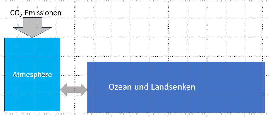5: The 2-box model</figcaption></figure>   This second box is$ k $times larger than the first box. To illustrate the effect, let us assume$ k=3 $. 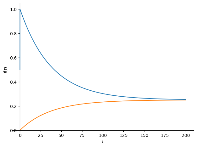It seems extreme that the oceans and land plants together are assumed to be only three times larger than the atmosphere. But this is actually the value assumed by current climate research (e.g., <a href="https://www.zdf.de/play/talk/markus-lanz-114/markus-lanz-vom-10-juli-2025-100">Prof. Marotzke on Markus Lanz TV show, July 10, 2025</a>, minute 21:30), even though it is known that <strong>the oceans alone have bound about 50 times as much CO₂ as the atmosphere</strong>. In the Bern model, the factor$ k $is closer to 4. If we imagine that the receiving container is actually only 3 times larger than the atmosphere, then it is also clear that, in the end, i.e., in a state of equilibrium, 25% of any additional CO₂ entering the atmosphere will remain in the atmosphere, and only 75% can be absorbed by the sinks. This is illustrated by the impulse response.   <figure class="wp-block-image size-full is-resized"><img src="https://klima-fakten.net/wp-content/uploads/2025/10/Unbenannt-1.png" alt="" class="wp-image-12079" style="width:939px;height:auto"/><figcaption class="wp-element-caption">Fig. 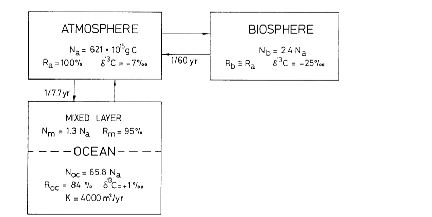6: 2-box model with k=3, Curve atmosphere (blue), Curve ocean (orange)</figcaption></figure>   The Bern model is a 4-box model. It divides the ocean into 2 parts. While in the upper part gas exchange occurs with a similar time constant as in the linear model (since only the uppermost layer, the ``mixed layer,'' is taken into account, the exchange is even faster than in the linear model), the flow into the deep sea occurs through very slow diffusion. The fourth box represents land plants. The fact that the deep sea is ``shielded'' for hundreds of years by the slow diffusion process explains the supposedly small ``ocean box'' and the resulting large constant residue of over 20% in the atmosphere.   <figure class="wp-block-image size-full"><img src="https://klima-fakten.net/wp-content/uploads/2025/12/image-12.png" alt="" class="wp-image-12519"/><figcaption class="wp-element-caption">Fig 7: The 4 boxes of the Bern model (Figure 1 from <a href="https://www.cambridge.org/core/services/aop-cambridge-core/content/view/S0033822200009449">https://www.cambridge.org/core/services/aop-cambridge-core/content/view/S0033822200009449</a>)</figcaption></figure>   <a href="https://acp.copernicus.org/articles/13/2793/2013/">The published approximation equation of the Bern model is</a>  $ IRF^{Bern}(t) =a_0 + \sum_{i=1}^3 a_i\cdot e^{-\frac{t}{\tau_i}} $(Equation 5)   with  $ a_0=0.21787, a_1=0.22896, a_2=0.28454, a_3=0.26863 $,  $ \tau_1=381.33, \tau_2=34.785, \tau_3=4.1237 $.   The mathematical form of the approximate solution and the cited publication suggest that there are four parallel processes. <strong>However, this is not the case; it is only <a href="https://tellusjournal.org/articles/2448/files/submission/proof/2448-1-45288-1-10-20221012.pdf">an approximate solution of a complex 4-box process</a></strong> in order to be able to formulate the process more simply as a weighted sum of linear processes.   Fig. 6 shows the impulse response functions (IRF) of the Bern model (orange) compared to the above linear model (green) and the 2-box model (magenta).   <figure class="wp-block-image size-full"><img src="https://klima-fakten.net/wp-content/uploads/2025/12/image-10.png" alt="" class="wp-image-12439"/><figcaption class="wp-element-caption">Fig. 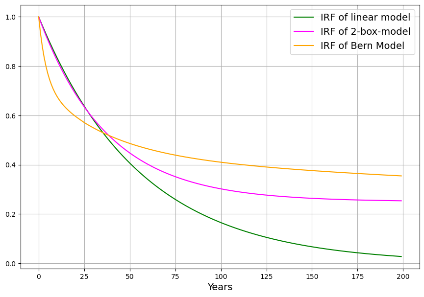8: The impuls response functions of the linear model (green), the 2-box model (magenta), and the Bern model (orange)</figcaption></figure>   While the decline in concentration is greater at the beginning of the Bern model than in the linear model, the curve soon flattens out so that after 100 years only 60% is absorbed, compared to 85% in the linear model. The 2-box model lies between the linear and Bern models in terms of its progression; in the long term, it reaches saturation in a similar way to the Bern model, i.e., a substantial proportion of the CO₂ remains in the atmosphere.   <h4 class="wp-block-heading">Application to the real emission curve</h4>   The decisive test is carried out using the actual measured data, the measured anthropogenic emissions according to Fig. 1.   Convolutions with the respective impulse responses described above result in the concentration curves of the two models and a natural equilibrium concentration of 285 ppm (Fig. 9). With the time series up to the end of 2024, the differences between the models in the reconstruction of the measured CO₂ concentration are very small (since the measurement data before 1960 are unreliable anyway, the deviations before 1960 are of minor interest). Between 1960 and 2020, not only do the two models agree with each other, but they also agree with the measured concentration data.   <figure class="wp-block-image size-full"><img src="https://klima-fakten.net/wp-content/uploads/2025/12/Unbenannt-6.png" alt="" class="wp-image-12353"/><figcaption class="wp-element-caption">Fig. 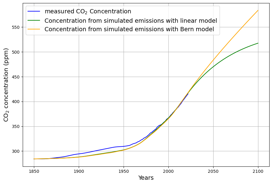9: Measured concentration curve (blue), reconstruction of the concentration with linear model (green), and reconstruction of concentration with Bern model (orange)</figcaption></figure>   However, it is clear from Fig. 9 that the sink effect of the Bern model diminishes significantly in the long term compared to the linear model and, as a result, the concentration increases more sharply from 2030 onwards than in the linear model. For this reason, the sink effect is calculated as a comparison criterion for both models in the same way as for the real measurement data.   The concentration growth is determined by calculating the difference between adjacent data points from the modeled concentration curve (equation (1)). The measured sink effect, which is important for the differentiation criterion, is determined from the difference between measured emissions and the concentration growth determined in this way according to equation (2). The respective sink effects determined from this are summarized in Figure 10.   <figure class="wp-block-image size-full is-resized"><img src="https://klima-fakten.net/wp-content/uploads/2025/12/image-11.png" alt="" class="wp-image-12445" style="width:960px;height:auto"/><figcaption class="wp-element-caption">Fig. 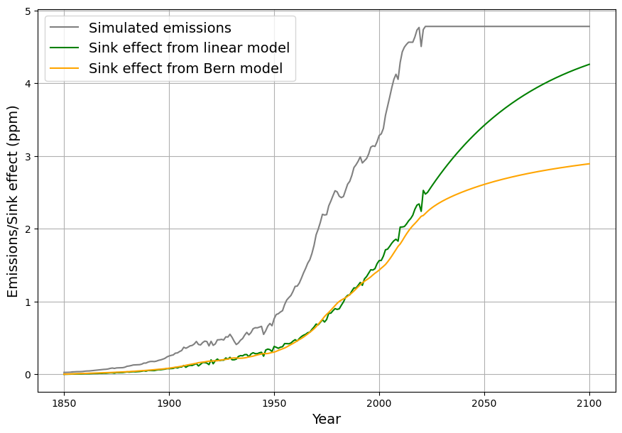10: Measured Emissions (grey), sink effect of linear model (green) , and sink effect of Bern model (orange)</figcaption></figure>   Once again, it is confirmed that the linear model and the Bern model differ only very slightly until 2020. However, the differences become very large thereafter, with the sink effect of the Bern model reaching near saturation (but not zero) by the end of the century, while the sink effect of the linear model approaches anthropogenic emissions in terms of the balance of sinks and sources as defined in the Paris Climate Agreement.   In order to be able to make a statement about the validity of the respective model today, a criterion is needed that allows a measurable difference in the respective sink effect to be determined from past data.   <h4 class="wp-block-heading">Criterion for distinguishing the linear model from the ``sink flattening'' model</h4>   Based on equation (4),<strong> the relative sink effect or sink ratio of any sink model at any point in time can be described by modifying the absorption constant$ a $of the linear model to a time-dependent variable$ a_i $</strong>:  $ S_i = a_i\cdot(C_{i-1} – C^0) $  The value of this time-dependent sink ratio$ a_i $is defined as the ratio of the sink effect$ S_i $derived from emissions and concentration growth to the concentration of the previous year<sup data-fn="63046410-c068-4c47-9f19-cc896b78554e" class="fn"><a href="#63046410-c068-4c47-9f19-cc896b78554e" id="63046410-c068-4c47-9f19-cc896b78554e-link">2</a></sup> exceeding the pre-industrial equilibrium concentration$ C^0 $ppm:  $ a_i = \frac{S_i}{C_{i-1}-C^0} = \frac{E_i – (C_i – C_{i-1})}{C_{i-1}-C^0} $  Consequently, the sink ratio$ a_i $is a variable that depends only on the measured anthropogenic emissions and the modeled or measured concentrations$ C_i $, apart from the constant$ C^0 $.   Fig. 11 shows these relative sink effects, the ``sink ratio''$ a_i$ for the linear model (green) and the Bern model (orange).

Fig. 11: Curve of sink ratio of linear model (green) and of Bern model (orange)

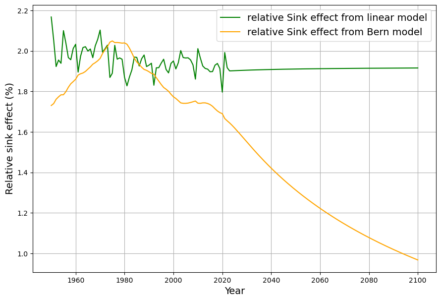
After a slight increase in the relative sink effect during the phase of exponential emissions growth until 1975, the Bern model shows a significant decline in the relative sink effect from 1980 onwards, while the relative sink effect in the linear model remains largely constant, as expected.

In order to obtain statistically evaluable measurement data from this graphical illustration using past data, the course of the relative sink effect over the 42-year period from 1980 to 2022 is approximated with a straight line in each case (Fig. 12):

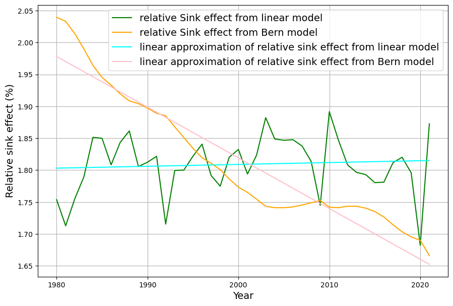
Fig. 12: Sink ratio of linear sink model (green) and its linear fit (turquois), sink ratio of Bern model (orange) and its linear fit (rose).

The trend of the two curves is well represented by the slope of the straight lines. The slope of these straight lines is therefore the significant distinguishing criterion between the two models. The least squares estimate of the straight line equation also gives the standard error of the slope. These two measured values are now plotted with their error distributions in a diagram (Fig. 13). In order to obtain a dimensionless result, the quotient of the slope and the expected value at the midpoint of the period is plotted and used as the relative slope (in %) as a value on the X-axis of Fig. 13. The diagram shows the probability distributions for the relative slope of both models.

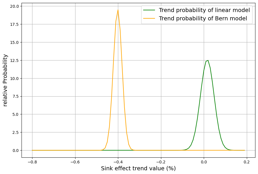
Fig. 13: Probability of sink ratio trend from 1980 to 2020 for linear model (green) and Bern model (orange)

The two probability distributions are so clearly disjoint that this provides a criterion in which the two models differ greatly, even over the last 40 years. In plain language, this means that there are hardly any trend deviations from the sink ratio of 0 in the linear model, while in the Bern model, there has been a trend since 1980 toward a relative reduction in the sink ratio of 0.4% per year, starting from a value that was still greater than in the linear model in 1980 but is already considerably lower now, as can be seen in Fig. 12.

The crucial question now, of course, is how the actual measured data behaves with regard to this criterion, and thus which of the two models is more consistent with the real data.

The sink ratio of the measured data

The decisive test is carried out with the actual measured data. With the time series up to the end of 2024, as shown in Fig. 9, the differences between the models in the reconstruction of the measured CO2 concentration are very small.

For this reason, the more meaningful curves of the measured sink effect are considered. In fact, slight differences are already apparent today. Since the measured sink effect (blue) is subject to extremely strong short-term fluctuations, these are smoothed (purple). This operation does not distort the long-term trend. For comparison, Fig. 14 shows the measured sink effect as annual “raw data” and as its smoothed curve in comparison to the linear and Berner models.

Fig. 14: Anthropogenic emissions (grey), yearly sink effect (blue), smoothed yearly sink effect (purple), linear sink model (green), Bern model (orange).

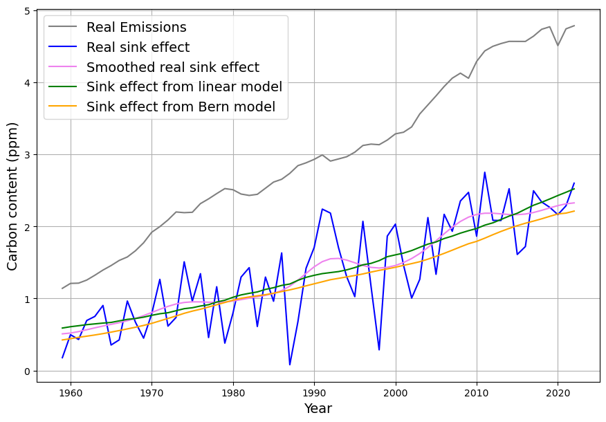
The model values of both models are still within the large statistical fluctuations of the measured sink effect as individual values. However, there are very slight differences in trends.

This is only clearly visible in the representation of the sink ratio or the relative sink effect in Fig. 15:

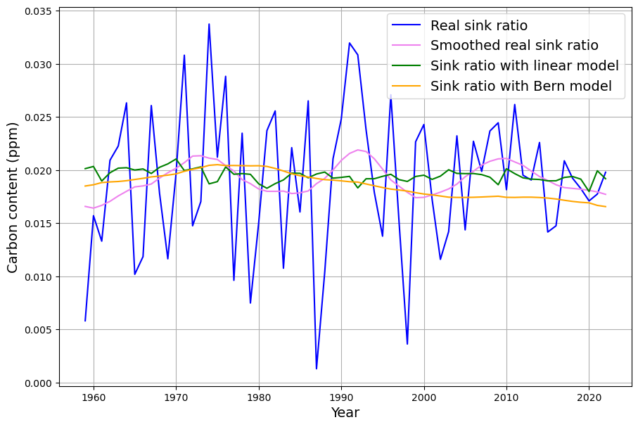
Fig. 15: Sink ratio of measured data (blue), sinkratio of measured data with smoothed sink effect (purple), sink ratio of linear model (green), sink ratio of Bern model (orange)

The sink ratio of the smoothed measured sink effect is approximated for the period 1980-2022 by a straight line whose slope is calculated with standard error and entered into a joint diagram (Fig. 16) with the results of the two models.

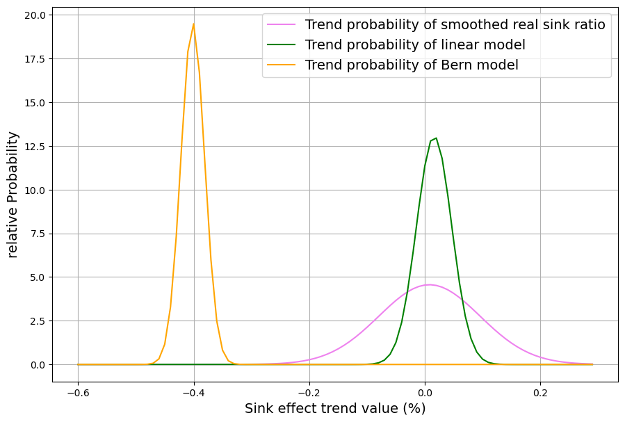
Fig. 16: Probability of sink ratio trend during 1980 to 2020 for measured, smoothed sink effect (purple), for linear sink model (green), and Bern model (orange)

The result is unambiguous. Only the linear sink model is compatible with the measured sink effect of the last four decades. Contrary to superficial appearances, the decline in the relative sink effect of the Bern model, which began in 1980, cannot be reconciled with the measured values. Accordingly, the Bern model is not compatible with reality.

The same applies to other models such as the budget model (where the deviation from reality is even greater than with the Bern model) and the 2-box model described above. Only the linear sink model can be reconciled with the real data from the last 45 years. A 2-box model in which the second box is not 3 times but, for example, 50 times larger than the first was not investigated. It is to be expected that such “almost linear” models are also compatible with the measured data.

Fußnoten

“It doesn’t matter how beautiful your theory is, it doesn’t matter how smart you are. If it doesn’t agree with experiment, it’s wrong.” (Richard Feynman) ↩︎
This is a simplification, in der publikation Evaluating the Effectiveness of Natural Carbon Sinks Through a Temperature-Dependent Model the expected value of the time lag is calculated as 15-18 months ↩︎

Do the carbon sinks fail? Or rather their models?

Introduction – the model dilemma

What are sinks? A formal description

The two sink models

The linear sink model

The sink ratio of the measured data

Fußnoten

Dr. Joachim Dengler

Leave a Reply Cancel reply

Introduction – the model dilemma

What are sinks? A formal description

The two sink models

The linear sink model

The sink ratio of the measured data

Fußnoten

Dr. Joachim Dengler

You might also like

How much CO2 will remain in the atmosphere?

Invariance of natural CO2 sources and sinks regarding long time temperatur trend

A Computational Model for CO2-Dependence on Temperature in the Vostok Ice cores

Leave a Reply Cancel reply