 by
by 
Introduction – How does the climate narrative work?
There is no doubt that there is a climate narrative propagated by scientists, the media and politicians according to which we are on a catastrophic course due to anthropogenic CO2 emissions, which can supposedly only be halted by reducing emissions to zero by 2050.
All those who contradict the narrative, even in subtle details, are blacklisted like lepers, even if they are renowned scientists, even Nobel Prize winners[1][2] – with devastating consequences for applications, publications or funding applications.
How is it possible to bring all the important universities, including the most renowned ones such as Harvard, MIT and Stanford, Oxford, Cambridge and Heidelberg, onto the same consensus line? How can the most famous journals such as Nature[3] and Science, as well as popular science journals such as Spektrum der Wissenschaft, only accept a narrow “tunnel of understanding” without obviously ruining their reputation?
In order for the narrative to have such a strong and universal impact, a solid scientific foundation is undoubtedly necessary, which cannot be disputed without embarrassment. Those who do so anyway are easily identified as “climate deniers” or “enemies of science”.
On the other hand, the predictions and, in particular, the political consequences are so misanthropic and unrealistic that not only has a deep social divide emerged, but an increasing number of contemporaries, including many scientists, are questioning what kind of science it is that produces such absurd results . [4]
A careful analysis of the climate issue reveals a pattern that runs like a red thread through all aspects. This pattern is illustrated in the example of 4 key areas that are important in climate research.
The pattern that has emerged from many years of dealing with the topic is that there is always a correct observation or a valid law of nature at the core. In the next step, however, the results of this observation are either extrapolated into the future without being checked, the results are exaggerated or even distorted in their significance. Other, relevant findings are omitted or their publication is suppressed.
The typical conclusion that can be drawn from the examples mentioned and many others is that each aspect of the climate threatens the most harmful outcome possible. The combination of several such components then leads to the catastrophic horror scenarios that we are confronted with on a daily basis. As the statements usually relate to the future, they are generally almost impossible to verify.
The entire argumentation chain of the climate narrative takes the following form:
- Anthropogenic emissions are growing – exponentially.
- Atmospheric concentration increases with emissions as long as emissions are not completely reduced to zero
- The increase in the concentration of CO2 in the atmosphere leads to a – dramatic – increase in the average temperature
- In addition, there are positive feedbacks when the temperature rises, and even tipping points beyond which reversal is no longer possible.
- Other explanations such as hours of sunshine or the associated cloud formation are ignored, downplayed or built into the system as a feedback effect.
- The overall effects are so catastrophic that they can be used to justify any number of totalitarian political measures aimed at reducing global emissions to zero.
A detailed examination of the subject leads to the conclusion that each of these points shows the pattern described above, namely that there is always a kernel of truth that is harmless in itself. The aim of this paper is to work out the true core and the exaggerations, false extrapolations or omissions of essential information.
1. anthropogenic emissions are growing – exponentially?
Everyone knows the classic examples of exponential growth, e.g. the chessboard that is filled square by square with double the amount of rice. Exponential growth always leads to disaster. It is therefore important to examine the facts of emissions growth.
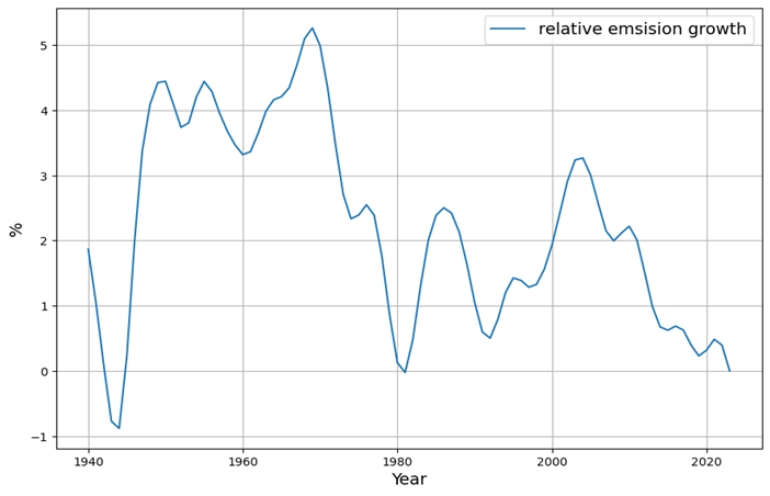
Figure 1 shows the relative growth of global anthropogenic emissions over the last 80 years. To understand the diagram, let us remember that constant relative growth means exponential growth[7] . A savings account with 3% interest grows exponentially in principle. Accordingly, we find exponential growth in emissions with a growth rate of around 4.5% between 1945 and 1975. This phase was once known as the “economic miracle”. After that, emissions growth fell to 0 by 1980. This period was known as the “recession”, which resulted in changes of government in the USA and Germany.
A further low point in the growth of emissions was associated with the collapse of communism around 1990, with a subsequent rise again, mainly in the emerging countries. Since 2003, there has been an intended reduction in emissions growth as a result of climate policy.
It should be noted that emissions growth has currently fallen to 0.
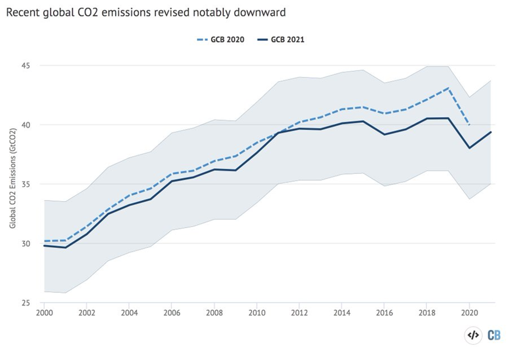
Recently, Zeke Hausfather found that the sum of global anthropogenic emissions since 2011 has been constant within the measurement accuracy[8] , shown in Figure 2.
As a result, current emissions are no longer expected to be exceeded in the future[9] .
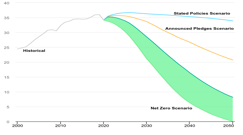
The longer-term extrapolation of the current planned future emissions, the so-called “Stated Policies” scenario (from 2021), expects constant global emissions until 2030 and a very slight reduction of 0.3% per year thereafter.
As a result, the two future scenarios most frequently used by the IPCC (RCP 8.5 and RCP6.2) are far removed from reality[12] of the emission scenarios that are actually possible. Nevertheless, the extreme scenario RCP8.5 is still the most frequently used in the model calculations . [13]
The IPCC scenario RCP4.5 and the similar IEA scenario “Stated Policies” shown in Figure 3 (p. 33, Figure 1.4) are the most scientifically sound .[14]
This means that if the realistic emission scenarios are recognized without questioning the statements about the climate disseminated by the IPCC, a maximum emission-related temperature increase of 2.5°C compared to pre-industrial levels remains.
2. atmospheric CO2 concentration increases continuously — unless emissions are reduced to zero?
The question is how anthropogenic emissions affect the CO2 concentration in the atmosphere. It is known and illustrated in Fig. 4 by the International Energy Agency that by no means all the CO2 emitted remains in the atmosphere, but that a growing proportion of it is reabsorbed by the oceans and plants.
The statistical evaluation of anthropogenic emissions and the CO2 concentration, taking into account the conservation of mass and a linear model of the natural sinks oceans and biosphere, shows that every year just under 2% of the CO2 concentration exceeding the pre-industrial natural equilibrium level is absorbed by the oceans and the biosphere.
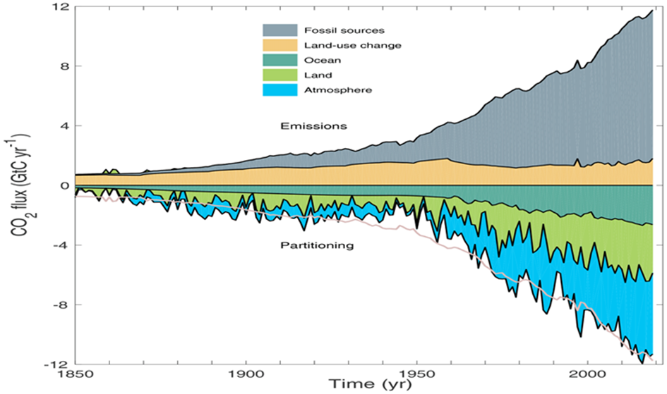
land sinks) and concentration growth in the atmosphere
are absorbed [15][16] . This is currently half of anthropogenic emissions and the trend is increasing, as shown in Figure 5.
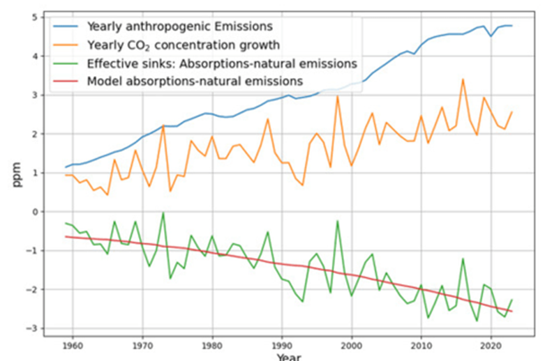
concentration growth (orange), natural sinks and their modeling (green)
The most likely global future scenario of the International Energy Agency – the extrapolation of current political regulations (Stated Policies Scenario STEPS) shown in Fig. 3 – includes a gentle decrease (3%/decade) in global emissions to the 2005 level by the end of the century. These emission reductions are achievable through efficiency improvements and normal progress.
If we take this STEPS reference scenario as a basis, using the linear sink model leads to an increase in concentration of 55 ppm to a plateau of 475 ppm, where the concentration then remains.
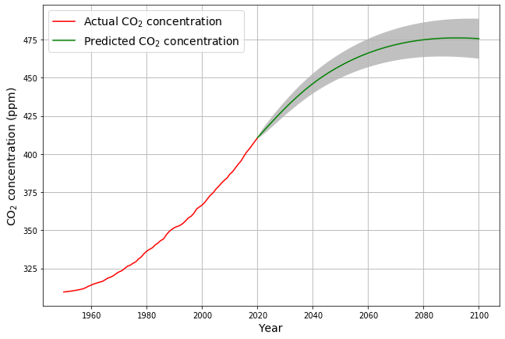
It is essential that the CO2 concentration does not rise to climatically dangerous levels. Article 4.1 of the Paris Climate Agreement[17]
states that countries must reach their maximum emissions as soon as possible “in order to achieve a balance between anthropogenic greenhouse gas emissions and removals by sinks in the second half of this century“. The Paris Climate Agreement therefore by no means calls for complete decarbonization.
The net-zero balance between emissions and absorption will be achieved in 2080 by extrapolating today’s behavior without radical climate measures.
Without going into the details of the so-called sensitivity calculation, the following can be simplified for the further temperature development:
Assuming that the CO2 concentration is fully responsible for the temperature development of the atmosphere, the CO2 concentration in 2020 was 410 ppm, i.e. (410-280) ppm = 130 ppm above the pre-industrial level. Until then, the temperature was about 1° C higher than before industrialization. In the future, we can expect the CO2 concentration to increase by (475-410) ppm = 65 ppm based on the above forecast. This is just half of the previous increase. Consequently, even if we are convinced of the climate impact of CO2 , we can expect an additional half of the previous temperature increase by then, i.e. ½° C. This means that by 2080, the temperature will be 1.5° C above pre-industrial levels, meeting the target of the Paris Climate Agreement, even without radical emission reductions.
3. atmospheric CO2 concentration causes – dramatic? – rise in temperature
After the discussion about possible future CO2 quantities, the question arises as to their impact on the climate, i.e. the greenhouse effect of CO2 and its influence on the temperature of the earth’s surface and the atmosphere.
The possible influence of CO2 on global warming is that its absorption of thermal radiation causes this radiation to be attenuated when it reaches outer space. The physics of this process is radiative transfer[18] . As the topic is fundamental to the entire climate debate on the one hand, but on the other hand demanding and difficult to understand, the complicated physical formulas are not used here.
In order to be able to measure the greenhouse effect, the infrared radiation emitted into space must be measured. However, the expected greenhouse effect of 0.2 W/m2 per decade[19] is so tiny that it is not directly detectable with today’s satellite technology, which has a measurement accuracy of around 10 W/m 2[20] .
We therefore have no choice but to make do
with mathematical models of the physical radiative transfer equation. However, this is not valid proof of the effectiveness of this CO2 greenhouse effect in the real, much more complex atmosphere.
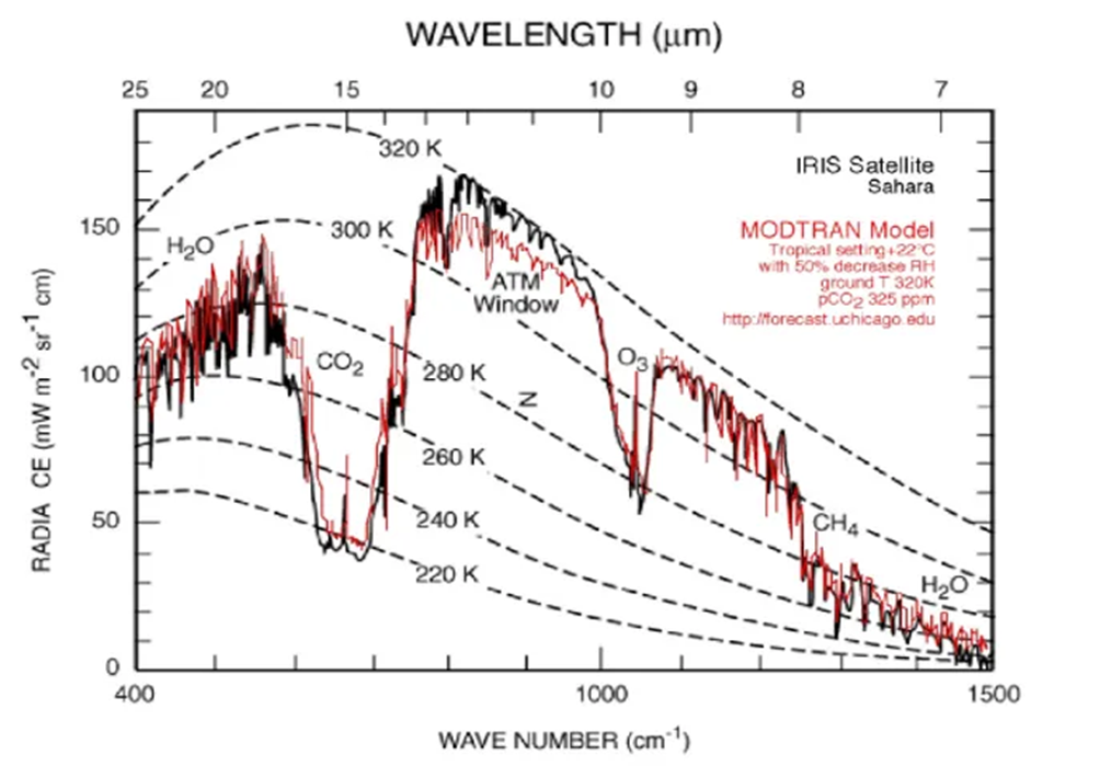
There is a widely recognized simulation program MODTRAN[21] , with which the radiation of infrared radiation into space and thus also the CO2 greenhouse effect can be physically correctly simulated:
Figure 7 shows that the MODTRAN reconstruction of the infrared spectrum is in excellent agreement with the infrared spectrum measured from space. We can thus justify the applicability of the simulation program and conclude that the simulation can also be used to describe hypothetical constellations with sufficient accuracy.
With this simulation program we want to check the most important statements regarding the greenhouse effect.
To start in familiar territory, we first try to reproduce the commonly published “pure CO2 greenhouse effect” by allowing the solar radiation, which is not reduced by anything, to warm the earth and its infrared radiation into space to be attenuated solely by the CO2 concentration. The CO2 concentration is set to the pre-industrial level of 280 ppm.
We use the so-called standard atmosphere[22] , which has proven itself for decades in calculations that are important for aviation, but remove all other trace gases, including water vapor. However, the other gases such as oxygen and nitrogen are assumed to be present, so that nothing changes in the thermodynamics of the atmosphere. By slightly correcting the ground temperature to 13.5°C (reference temperature is 15°C), the infrared radiation is set to 340 W/m2 . This is just ¼ of the solar constant[23] , so it corresponds exactly to the solar radiation distributed over the entire surface of the earth.
The “CO2 hole”, i.e. the reduced radiation in the CO2 band compared to the normal Planck spectrum[24] , is clearly visible in the spectrum.
What happens if the CO2 concentration doubles?
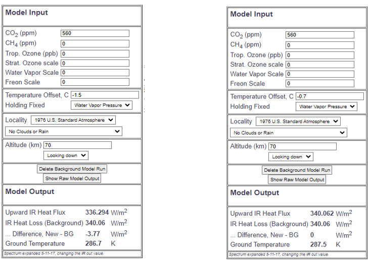
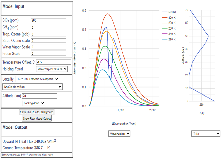
Illustration 9 Radiative forcing in Figure 9a Temperature increase for
CO2 doubling (no albedo, compensation of radiative forcing
no water vapor) from Fig. 9.
Fig. 9 shows that doubling the CO2 concentration to 560 ppm reduces the heat flux of infrared radiation by 3.77 W/m2 . This figure is used by the IPCC and almost all climate researchers to describe the CO2 forcing. In Fig. 9a, we change the ground temperature from -1.5°C to -0.7°C in order to achieve the radiation of 340 W/m2 again. This warming of 0.8°C with a doubling of the CO2 concentration is referred to as “climate sensitivity”. It is surprisingly low given the current reports of impending climate catastrophes.
Especially when we consider that the settings of the simulation program used so far are completely at odds with the real Earth’s atmosphere:
- No consideration of the albedo, the reflection of light,
- No consideration of clouds and water vapor
We will now approach the real conditions step by step. The scenarios are summarized in Table 1:
| Scenario | Albedo | Irradiation (W/m )2 | CO2 before (ppm) | Temperature ( °C) | CO2 after (ppm) | Drive (W/m )2 | Temperature Increase for balance (°C) |
| Pre-industrial CO only2 , no clouds, No water vapor | 0 | 340 | 280 | 13,7 | 560 | -3,77 | 0,8 |
| No greenhouse gases, No clouds (CO 2 from 0-280 ppm) | 0,125 | 297,5 | 0 | -2 | 280 | -27 | 7 |
| CO only2 , Albedo, no clouds, No water vapor | 0,125 | 270 | 280 | 5 | 560 | -3,2 | 0,7 |
| Pre-industrial standard atmosphere | 0,3 | 240 | 280 | 15 | 560 | -2 | 0,5 |
| Pre-industrial standard atmosphere, CO2 today Concentration | 0,3 | 240 | 280 | 15 | 420 | -1,1 | 0,3 |
The scenario in the first row of Table 1 is the “pure CO2 ” scenario just discussed.
In the second line, we go one step back and also remove the CO2 , i.e. a planet without greenhouse gases, without clouds, without water vapor. But the Earth’s surface reflects sunlight, so it has an albedo[25] . The albedo value of 0.125 corresponds to that of other rocky planets as well as the ocean surface. Surprisingly, in this case the surface temperature is -2°C (and not -18°C as is often claimed!). This is because there is no cloud albedo without water vapor. If the CO2 concentration is now increased to the pre-industrial level of 280 ppm, the infrared radiation is reduced by 27 W/m2 . This large radiative forcing is offset by a temperature increase of 7°C.
We can see that there is a considerable greenhouse effect between the situation without any greenhouse gases and the pre-industrial state, with a warming of 7°C.
The third line takes this pre-industrial state, i.e. Earth’s albedo, 280 ppm CO2 , no clouds and no water vapor, as the starting point for the next scenario. If the CO2 concentration is doubled, the radiative forcing is -3.2 W/m2 , i.e. slightly less than in the first “pure CO2 scenario”. As a result, the warming of 0.7°C to achieve radiative equilibrium is also slightly lower here.
After these preparations, the pre-industrial standard atmosphere with albedo, clouds, water vapor and the real measured albedo of 0.3 is represented in the 4th row, with the ground temperature of 15°C corresponding to the standard atmosphere. There are now several ways to adjust cloud cover and water vapor in order to achieve the infrared radiation of 340 W/m 2. (1-a) = 240 W/m2 corresponding to the albedo a=0.3. The exact choice of these parameters is not important for the result as long as the radiation is 240 W/m2 .
In this scenario, doubling the CO2 concentration to 560 ppm causes a radiative forcing of -2 W/m2 and a compensating temperature increase, i.e. sensitivity of 0.5°C.
In addition to the scenario of a doubling of the CO2 concentration, it is of course also interesting to see what the greenhouse effect has achieved to date. The current CO2 concentration of 420 ppm is just in the middle between the pre-industrial 280 ppm and double that value.
In the 5th row of the table, the increase from 280 ppm to 420 ppm causes the radiative forcing of -1.1 W/m2 and the temperature increase of 0.3°C required for compensation. From this result it follows that since the beginning of industrialization, the previous increase in CO2 concentration was responsible for a global temperature increase of 0.3°C.
This is much less than the average temperature increase since the beginning of industrialization. The question therefore arises as to how the “remaining” temperature increase can be explained.
There are several possibilities:
- Positive feedback effects that intensify CO2 -induced warming. This is the direction of the Intergovernmental Panel on Climate Change and the topic of the next chapter.
- Other causes such as cloud albedo. This is the subject of the next but one chapter
- Random fluctuations. In view of the chaotic nature of weather events, chance is often used. This possibility remains open in the context of this paper.
4. feedback leads to — catastrophic? — consequences
The maximum possible climate sensitivity in the previous chapter, i.e. temperature increase with a doubling of the CO2 concentration, is 0.8°C, under real conditions rather 0.5°C.
It was clear early on in climate research that such low climate sensitivity could not seriously worry anyone in the world. In addition, the measured global warming is greater than predicted by the radiative transfer equation.
This is why feedbacks were brought into play; the most prominent publication in this context was by James Hansen et al. in 1984: “Climate Sensitivity: Analysis of Feedback Mechanisms”[26] (Climate Sensitivity: Analysis of Feedback Mechanisms). It was James Hansen who significantly influenced US climate policy with his appearance before the US Senate in 1988[27] . Prof. Levermann made a similar argument at a hearing of the German Bundestag’s Environment Committee[28] , claiming that the temperature would rise by 3°C due to feedback.
The high sensitivities published by the IPCC for a doubling of the CO2 concentration between 1.5°C and 4.5°C arose with the help of the feedback mechanisms.
In particular, the question arises as to how a small warming of 0.8°C can lead to a warming of 4.5°C through feedback without the system getting completely out of control?
By far the most important feedback in this context is the water vapor feedback.
How does water vapor feedback work?
The water vapor feedback consists of a 2-step process:
- If the air temperature rises by 1°C, the air can absorb 6% more water vapor[29] . It should be noted that this percentage is the maximum possible water vapor content. Whether this is actually achieved depends on whether sufficient water vapor is available.
- The radiation transport of infrared radiation depends on the relative humidity:
Additional humidity reduces the emitted infrared radiation as a result of absorption by the additional water vapor.
Using the MODTRAN simulation program already mentioned, the reduction of infrared radiation by 0.69 W/m2 is determined by increasing the humidity by 6%, e.g. from 80% to 86%[30] .
This reduced infrared radiation is a negative radiative forcing. The temperature increase compensating for this attenuation is the primary feedback g (“gain”). This is 0.19°C as a result of the original temperature increase of 1°C, i.e. g=0.19.
The total feedback f results as a geometric series[31] due to the recursive application of the above mechanism – the 0.19°C additional temperature increase results in further additional water vapor formation. This relationship is described by James Hansen in his 1984 paper[32] :
f = 1+ g + g2 + g3 … = 1/(1-g).
With g=0.19, the feedback factor f = 1.23.
Assuming a greenhouse effect from radiative transfer of 0.8°C, together with the maximum possible feedback, this results in a temperature increase of
0.8°C. 1.23 = 0.984 °C 1°C, with the sensitivity determined here of 0.5°C. 1.23 = 0.62 °C.
Both values are lower than the lowest published sensitivity of 1.5°C of the models used by the IPCC.
The warming that has occurred since the beginning of industrialization is therefore 0.3°C. 1.23 = 0.37°C even with feedback.
This proves that even the frequently invoked water vapor feedback does not lead to exorbitant and certainly not catastrophic global warming.
5. but it is warming up? – Effects of clouds.
To stop at this point will leave anyone dealing with the climate issue with the obvious question: “But the earth is warming, and more than would be possible according to the revised greenhouse effect including feedback?”.
For this reason, the effects of actual cloud formation, which until recently have received little attention in the climate debate, are examined here[33] .
Investigation of changes in global cloud cover
Jay R Herman from NASA[34] has calculated and evaluated the average reflectivity of the Earth’s cloud cover with the help of satellite measurements over a period of more than 30 years:
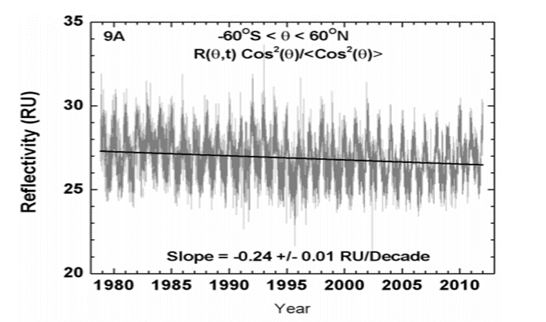
He identified a clear trend of decreasing cloud cover. From this he calculated, how this affects the affected components of the global energy budget:
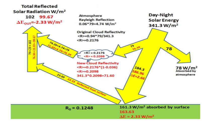
The result was that due to the reduced cloud cover, solar radiation increased by 2.33 W/m2 in 33 years. That is 0.7 W/m2 of radiative forcing per decade. In contrast, the decrease in radiation due to the increase in CO2 concentration amounted to a maximum of 0.2 W/m2 per decade . [35]
According to this study, at 78% the influence of clouds on the climate is at least 3.5 times greater than that of CO2 , which therefore has an influence of 22% at most.
Conclusion – there is no impending climate catastrophe
Let us summarize the stages of these observations on the deconstruction of the climate narrative once again:
- There is no exponential growth in CO2 emissions. This phase existed until 1975, but it is long gone and global emissions have reached a plateau in the last 10 years.
- The CO2 concentration is still growing despite constant emissions, but its growth has already slowed and will stop in the second half of the century assuming the most likely emissions scenario.
- The physically plausible greenhouse effect of CO2 is much lower than is usually claimed; the sensitivity that can be justified under real atmospheric conditions is only 0.5°C.
- Estimating the maximum possible feedback effect of water vapor results in the upper limit of the feedback factor as 1.25. This does not justify temperature increases of 3°C or more
- There are plausible simple explanations for the earth’s temperature development. The most important of these is that, as a result of various air pollution control measures (reduction of wood and coal combustion, catalytic converters in cars, etc.), aerosols in the atmosphere have decreased over the last 70 years, which has led to a reduction in cloud formation and therefore to an increase in solar radiation.
Footnotes
[1]https://www.eecg.utoronto.ca/~prall/climate/skeptic_authors_table.html
[2]https://climatlas.com/tropical/media_cloud_list.txt
[3]https://www.cfact.org/2019/08/16/journal-nature-communications-climate-blacklist/
[4]e.g. https://clintel.org/
[5]Raw data: https://ourworldindata.org/co2-emissions
[6]Relative growth: https://www.statisticshowto.com/relative-rate-of-change-definition-examples/#:~:text=Relative%20rates%20of%20change%20are,during%20that%20ten%2Dyear%20interval.
[7]https://www.mathebibel.de/exponentielles-wachstum
[8]https://www.carbonbrief.org/global-co2-emissions-have-been-flat-for-a-decade-new-data-reveals/
[9]https://www.carbonbrief.org/analysis-global-co2-emissions-could-peak-as-soon-as-2023-iea-data-reveals/
[10]https://www.carbonbrief.org/global-co2-emissions-have-been-flat-for-a-decade-new-data-reveals/
[11]https://www.iea.org/data-and-statistics/charts/co2-emissions-in-the-weo-2021-scenarios-2000-2050
[12]https://www.nature.com/articles/d41586-020-00177-3
[13]https://rogerpielkejr.substack.com/p/a-rapidly-closing-window-to-secure
[14]https://iea.blob.core.windows.net/assets/4ed140c1-c3f3-4fd9-acae-789a4e14a23c/WorldEnergyOutlook2021.pdf
[15]https://judithcurry.com/2023/03/24/emissions-and-co2-concentration-an-evidence-based-approach/
[16]https://www.mdpi.com/2073-4433/14/3/566
[17]https://eur-lex.europa.eu/legal-content/DE/TXT/?uri=CELEX:22016A1019(01)
[18]http://web.archive.org/web/20210601091220/http:/www.physik.uni-regensburg.de/forschung/gebhardt/gebhardt_files/skripten/WS1213-WuK/Seminarvortrag.1.Strahlungsbilanz.pdf
[19]https://www.nature.com/articles/nature14240
[20]https://www.sciencedirect.com/science/article/pii/S0034425717304698
[21]https://climatemodels.uchicago.edu/modtran/
[22]https://www.dwd.de/DE/service/lexikon/Functions/glossar.html?lv3=102564&lv2=102248#:~:text=In%20der%20Standardatmosph%C3%A4re%20werden%20die,Luftdruck%20von%201013.25%20hPa%20vor.
[23]https://www.dwd.de/DE/service/lexikon/Functions/glossar.html?lv3=102520&lv2=102248#:~:text=Die%20Solarkonstante%20ist%20die%20Strahlungsleistung,diese%20Strahlungsleistung%20mit%20ihrem%20Querschnitt.
[24]https://de.wikipedia.org/wiki/Plancksches_Strahlungsgesetz
[25]https://wiki.bildungsserver.de/klimawandel/index.php/Albedo_(simple)
[26]https://pubs.giss.nasa.gov/docs/1984/1984_Hansen_ha07600n.pdf
[27]https://www.hsgac.senate.gov/wp-content/uploads/imo/media/doc/hansen.pdf
[28]https://www.youtube.com/watch?v=FVQjCLdnk3k&t=600s
[29]A value of 7% is usually given, but the 7% is only possible from an altitude of 8 km due to the reduced air pressure there.
[30]h ttps://klima-fakten.net/?p=9287
[31]https://de.wikipedia.org/wiki/Geometrische_Reihe
[32]https://pubs.giss.nasa.gov/docs/1984/1984_Hansen_ha07600n.pdf
[33]The IPCC generally treats clouds only as potential feedback mechanisms.
[34]https://www.researchgate.net/publication/274768295_A_net_decrease_in_the_Earth%27s_cloud_aerosol_and_surface_340_nm_reflectivity_during_the_past_33_yr_1979-2011
[35]https://www.nature.com/articles/nature14240
Dear Dr. Dengler:
I have been analyzing our climate for a decade, or so, and it has led me to the conclusion that CO2 is a harmless gas that has NO climatic effect (apart from a decreasing albedo because of its greening of our planet).
This is explained in my recent article “Scientific proof that CO2 does NOT cause global warming”.
https://wjarr.com/sites/default/files/WJARR-2024-0884.pdf
My conclusions are irrefutable, although you are welcome to try.
Thank you for your comment.
I am not trying to refute your conclusions, because my conclusions, as you can see, are similar to yours. As a matter of fact I had seen your article before. But, to be honest, I am missing the scientific substance in your article. There is an introduction, and without detailled elaboration nor data handling and discussion, the conclusions. That cannot be taken serious by others, certainly not by those who you may want to convince.
Let me give you an example of an article with substance, that arrives at similar conclusions as you do: https://www.mdpi.com/2073-4433/12/10/1297