A Computational Model for CO2-Dependence on Temperature in the Vostok Ice cores

[latexpage]

The Vostok Ice core provides a more than 400000 year view into the climate history with several cycles between ice ages and warm periods.

It hat become clear that CO₂ data are lagging temperature data by several centuries. One difficulty arises from the necessity that CO₂ is measured in the gas bubbles whereas temperature is determined from a deuterium proxy in the ice. Therefore there is a different way of determining the age for the two parameters – for CO₂ there is a „gas age“, whereas the temperature series is assigned an „ice age“. There are estimates of how much older the „ice age“ is in comparison to the gas age. But there is uncertainty, so we will have to tune the relation between the two time scales.

Preprocessing the Vostok data sets

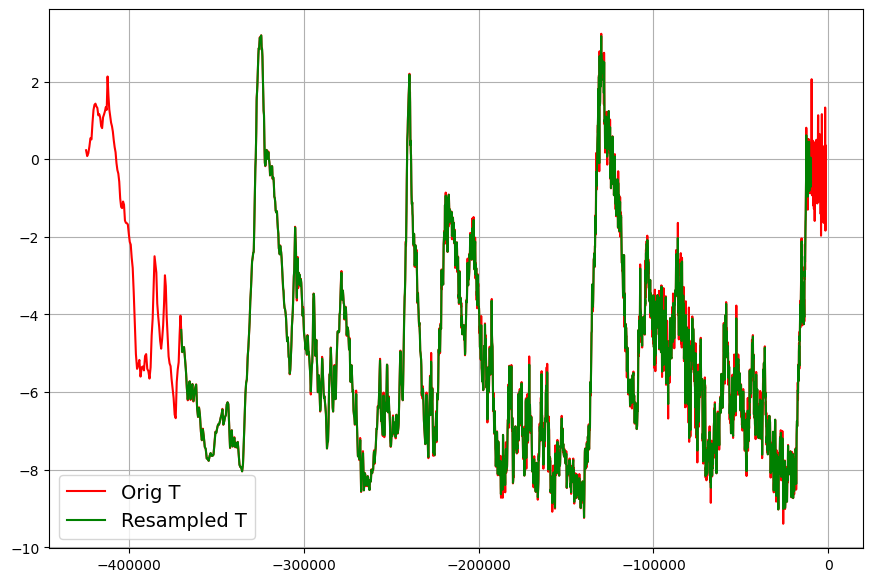
In order to perform model based computations with the two data sets, the original data must be converted into equally spacially sampled data sets. This is done by means of linear interpolation. The sampling interval is chosen 100 years, which is approximately the sampling interval of the temperature data. Apart from this, the data sets must be reversed, and the sign of the time axis must be set to negative values.
Here is the re-sampled temperature data set from -370000 years to -10000 years overlayed over the original temperature data:

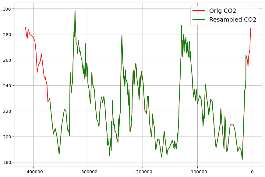
And here the corresponding CO₂-data set:

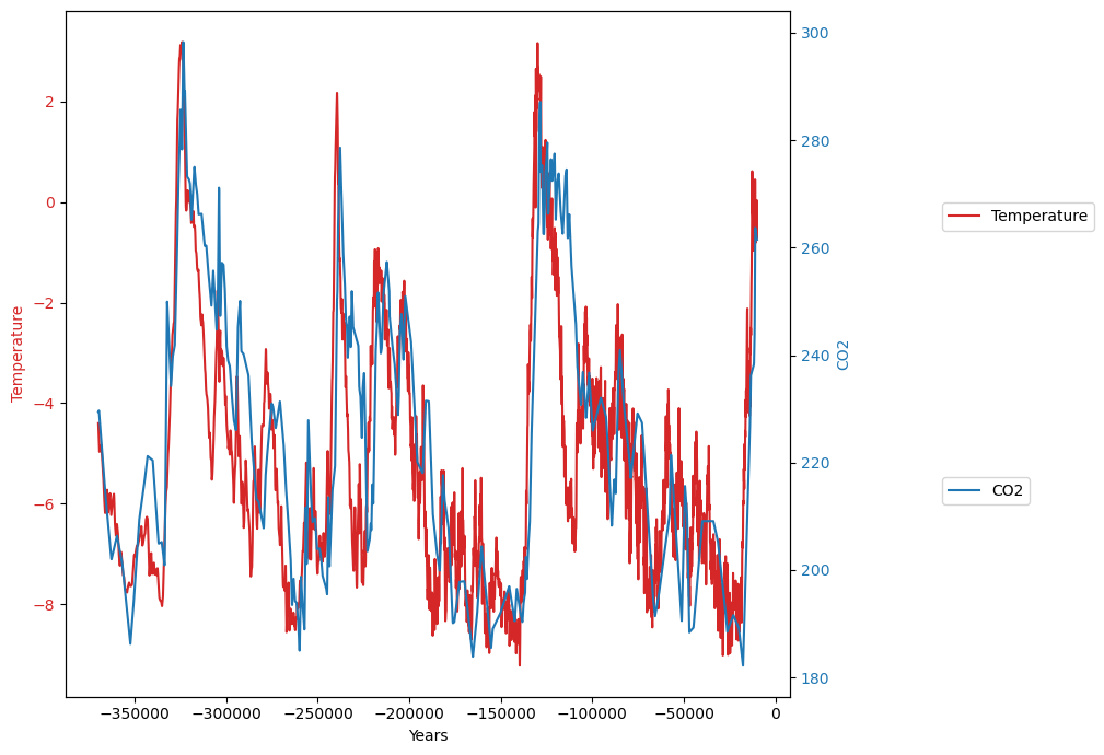
The two data sets are now superimposed:

Data model

Due to the fact of the very good predictive value of the temperature dependent sink model for current emission, concentration, and temperature data (equation 2) , we will use the same model based on CO₂ mass balance, and possible linear dependence of CO₂ changes on concentration and temperature, but obviously without the anthropogenic emissions. Also the time interval is no longer a single year, but a century.

G$_i$ is growth of CO₂-concentration C$_i$ during century i:

$G_i = C_{i+1}- C_i$

T$_i$ is the average temperature during century i. The model equation without anthropogenic emissions is:

$ – G_i = x1\cdot C_i + x2\cdot T_i + const$

After estimating the 3 parameters x1, x2, and const from G$_i$, C$_i$, and T$_i$ by means of ordinary least Squares, the modelled CO$_2$ data $\hat{C_i}$ are recursively reconstructed by means of the model, the first actual concentration value of the data sequence $C_0$, and the temperature data:
$\hat{C_0} = C_0$
$ \hat{C_{i+1}} = \hat{C_i} – x1\cdot \hat{C_i} – x2\cdot T_i – const$

Results – reconstructed CO$_2$ data

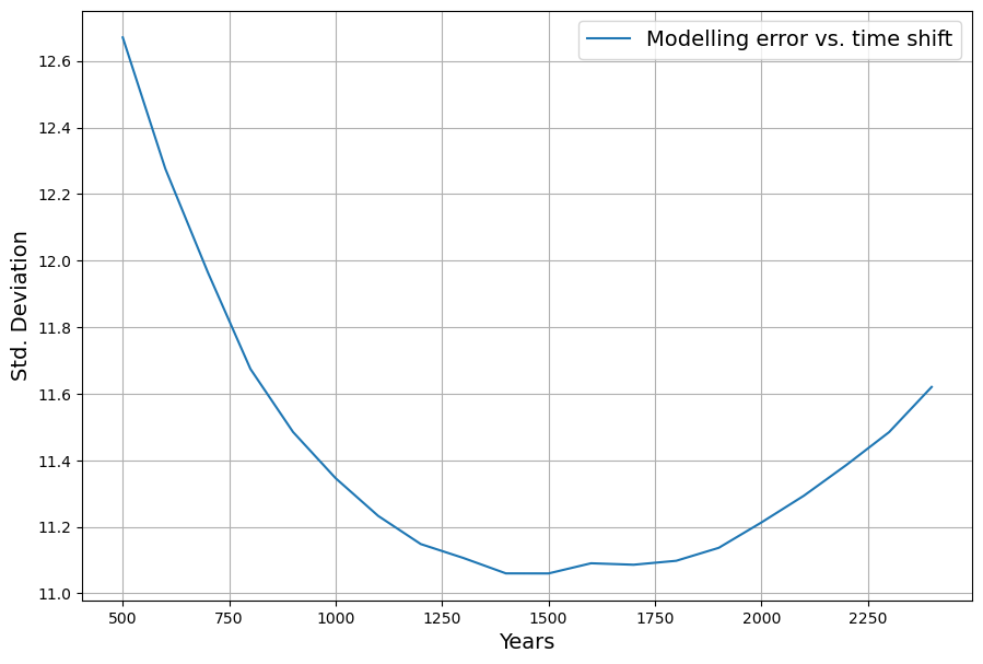
The standard deviation of $\{\hat{C_i}-C_i\}$ measures the quality of the reconstruction. Minimizing this standard deviation by shifting the temperature data is optimized, when the temperature data is shifted 1450..1500 years to the past:

Here are the corresponding estimated model parameters and the statistical quality measures from the Python OLS package:

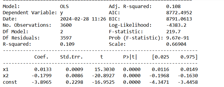
The interpretation is, that there is a carbon sink of 1.3% per century, and an emission increase of 0.18 ppm per century and 1 degree temperature increase.

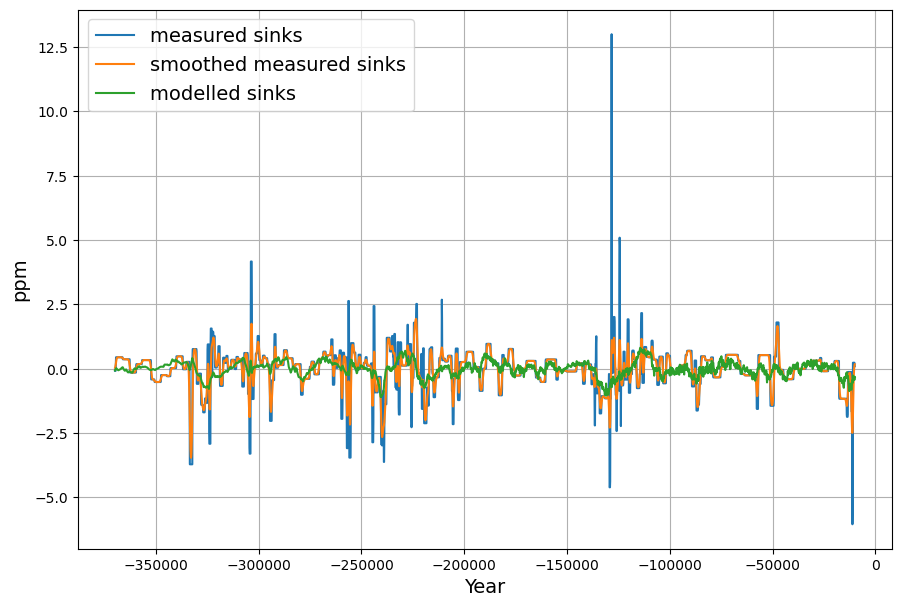
Modelling the sinks (-G$_i$) results in this diagram:

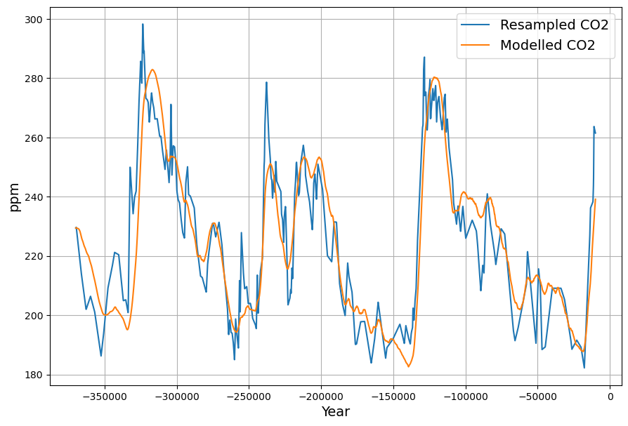
And the main result, the reconstruction of CO$_2$ data from the temperature extended sink modell looks quite remarkable:

Equilibrium Relations

The equilibrium states are more meaningful than the incremental changes. The equlibrium is defined by equality of CO2 sources and sinks, resulting in $G_i = 0$. This creates a linear relation between CO2 concentration C and Temperature T:

$C = \frac{0.1799\cdot T + 3.8965}{0.0133}$ ppm

For the temperature anomaly $T=0$ we therefore get the CO2 concentration of

$C_{T=0}=\frac{3.8965}{0.0133} ppm = 293 ppm$.
The difference of this to the modern data can be explained by different temperature references. Both levels are remarkably close, considering the very different environmental conditions.

And relative change is
$\frac{dC}{dT} = 13.5 \frac{ppm}{^\circ C} $

This is considerably different from the modern data, where we got $ 66.5 \frac{ppm}{°C}$.
There is no immediate explanation for this deviation. We need, however, consider the fact that we have time scale differences of at least 100 if not more. Therefore we can expect totally different mechanisms at work.