Global Temperature predictions
[latexpage]
Questioning the traditional approach
The key question to climate change is how much does the $CO_2$ content of the atmosphere influence the global average temperature? And in particular, how sensitive is the temperature to changes in $CO_2$ concentration?
We will investigate this by means of two data sets, the HadCRUT4 global temperature average data set, and the CMIP6 $CO_2$ content data set.
The correlation between these data is rather high, so it appears to be fairly obvious, that rising $CO_2$ content causes rising temperatures.
With a linear model it appears easy to find out how exactly temperatures at year i $T_i$ is predicted by $CO_2$ content $C_i$ and random (Gaussian) noise $\epsilon_i$. From theoretical considerations (radiative forcing) it is likely that the best fitting model is with $log(C_i)$:
$T_i = a + b\cdot log(C_i) + \epsilon_i$
The constants a and b are determined by a least squares fit (with the Python module OLS from package statsmodels.regression.linear_model):
a=-16.1, b=2.78
From this we can determine the sensitivity, which is defined as the temperature difference when $CO_2$ ist doubled:
$\Delta(T) = b\cdot log (2) °C = 1.93 °C $
This is nearly 2 °C, a number close to the official estimates of the IPCC.
What is wrong with this, it appears to be very straightforward and logical?
We have not yet investigated the residue of the least squares fit. Our model says that the residue must be Gaussian noise, i.e. uncorrelated.
The statistical test to measure this is the Ljung-Box test. Looking at the Q-criterion of the fit, it is Q = 184 with p=0. This means, that the residue has significant correlations, there is structural information in the residue, which has not been covered with the proposed linear model of log($CO_2$) content. Looking at the diagram which shows the fitted curve, we get a glimpse why the statistical test failed:
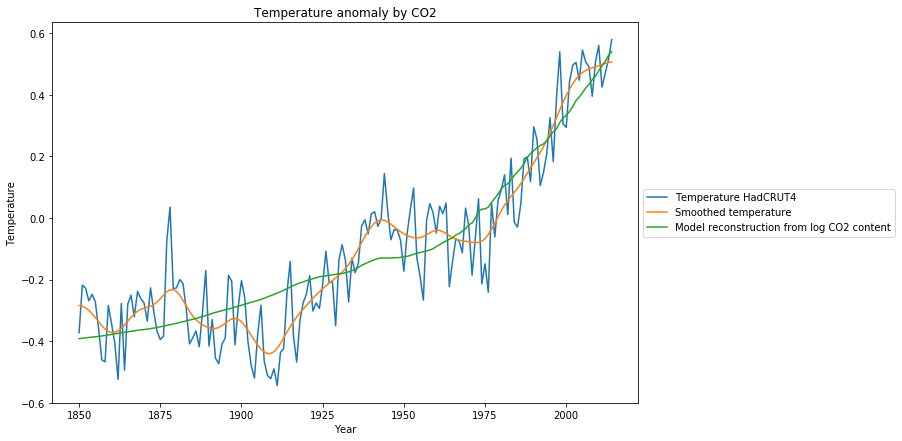
We see 3 graphs:
- The measured temperature anomalies (blue),
- the smoothed temperature anomalies (orange),
- the reconstruction of the temperature anomalies based on the model (green)
While the fit looks reasonable w.r.t. the noisy original data, it is obvious from the smoothed data, that there must be other systematic reasons for temperature changes besides $CO_2$, causing temporary temperature declines as during 1880-1910 or 1950-1976. Most surprizingly, from 1977-2000 the temperature rise is considerably larger than would be expected from the model of the $CO_2$ increase.
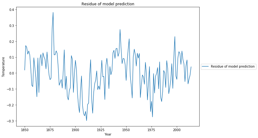
The systematic model deviations, among others a 60 year cyclic pattern, can also be observed when we look at the residue of the least squares fit:
Enhancing the model with a simple assumption
Considering the fact that the oceans and to some degree the biosphere are enormeous heat stores, which can take up and return heat, we enhance the temperature model with a memory term of the past. Not knowing the exact mechanism, this way we can include the „natural variability“ into the model. In simple terms this corresponds to the assumption: The temperature this year is similar to the temperature of last year. Mathematically this is modelled by an extended autoregressive process ARX(n),, where the Temperature at year i is assumed to be a sum of
- a linear function of the logarithm of the $CO_2$ content,log($C_i$), with offset a and slope b,
- a weighted sum of the temperature of previous years,
- random (Gaussian) noise $\epsilon_i$
$ T_i = a + b\cdot log(C_i) + \sum_{k=1}^{n} c_k \cdot T_{i-k} +\epsilon_i $
In the most simple case ARX(1) we get
$ T_i = a + b\cdot log(C_i) + c_1\cdot T_{i-1} +\epsilon_i $
With the given data the parameters are estimated, again with the Python module OLS from package statsmodels.regression.linear_model:
$a=-7.33, b=1.27, c_1=0.56 $
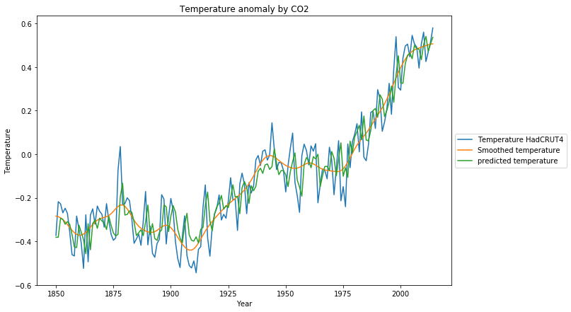
The reconstruction of the training data set is much closer to the original data:
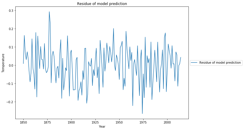
The residue of the fit now looks much more like a random process, which is confirmed by the Ljung-Box test with Q=20.0 and p=0.22
By considering the natural variability the sensitivity to $CO_2$ is reduced to
$\Delta(T) = b\cdot log (2) °C = 0.88 °C $
In another post we have applied the same type of model to the dependence of the atmospheric $CO_2$ content on the anthropogenic $CO_2$ emissions, and used this as a model for predictions of future atmospheric $CO_2$ content. 3 scenarios are investigated:
- „Business as usual“ re-defined from latest emission data as freezing global $CO_2$ emissions to the level of 2019 (which is what is actually happening)
- 100% worldwide decarbonization by 2050
- 50% worldwide decarbonization by 2100
The resulting atmospheric $CO_2$ has been calculated as follows:
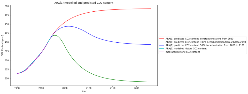
Feeding these predicted $CO_2$ content time series into the temperature ARX(1) model, the following global temperature scenarios can be expected for the future:
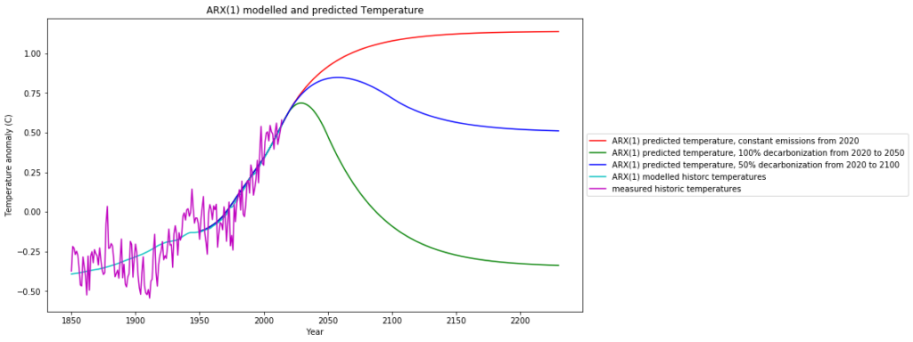
Conclusions
The following conclusions are made under the assumption that there is in fact a strong dependence of the global temperature on the atmospheric $CO_2$ content. I am aware that this is contested, and I myself have argued at other places that the $CO_2$ sensitivity is as low as 0.5°C and that the influence of cloud albedo is much larger than that of $CO_2$. Nevertheless it is worth taking the mainstream assumptions serious and take a look at the outcome.
Under the „business as usual“ scenario, i.e. constant $CO_2$ emissions at the 2019 level, we can expect a further temperature increase by appr. 0.5°C by 2150. This is 1.4°C above pre-industrial level and therefore below the 1.5° C mark of the Paris climate agreement.
Much more likely and realistic is the „50% decarbonization by 2100“ scenario, with a further 0.25°C increase, followed by a decrease to current temperature levels.
The politically advocated „100% decarbonization by 2050“, which is not only completely infeasible without economic collapse of most industrial countries, brings us back to the cold pre-industrial temperature levels which is not desireable.