Climate Sensitivity

[latexpage]

The central question of the whole climate discussion revolves around a single issue: how does the climate, in particular the world average temperature, change if the $CO_2$ content of the atmosphere doubles. This is called climate sensitivity, the adjusting screw of all climate policy. Based on the different modeling assumptions of the International Panel on Climate Change, the IPCC, we are threatened with an average temperature increase of 2°-5° C by the end of the century. The political „optimal target“ of the Paris climate agreement is a limit of 1.5° C.
The problem is that the resulting targets in terms of $CO_2$ avoidance are based on an assumed climate sensitivity of 2°-5° C with a doubling of $CO_2$.

Is this correct? Immense costs, the loss of industrial strength and the impoverishment caused by it, not least our freedom depend on the correct answer to this question.

A simple climate model

We want to use the well-established MODTRAN simulation as a one-dimensional mini-climate model to answer the question of climate sensitivity. MODTRAN incorporates a well accepted radiative transfer model. This simplification is legitimate in that the radiative equilibrium can in principle be calculated at any location on Earth, and if a consistent final result emerges under the various conditions, then we consider it reliable. The program is publicly available, so everything is verifiable. At this point we limit ourselves to an example calculation with the standard atmosphere, which is considered to be the optimal global average.

To do this, we set the MODTRAN program as the atmosphere had been in 1850 or so, in particular the $CO_2$ content was 280 ppm at that time. All other air constituents remain at the preset „standard“ average value. The atmosphere model is the so-called US Standard Atmosphere, as used in International Aviation. As cloud model I chose those clouds which are most common, the cumulus clouds between 660m and 2700m altitude. The water vapor content is then adjusted so that the outgoind infrared radiation just gets the correct value of about 240 $\frac{W}{m^2}$ (corresponding to the average equilibrium insolation with an average albedo of 0.3). This is given with an average relative water vapor content of 0.25. The assumed average surface temperature of the standard atmosphere is 15.2° C.

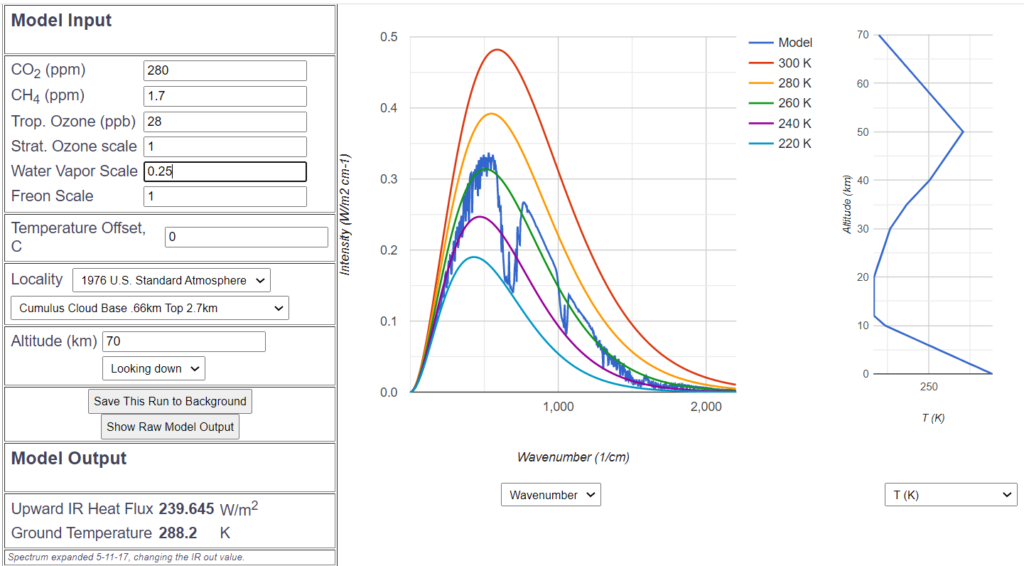
The dark blue spectrum shows the well known $CO_2$ hole, the influence of water vapor at both right and left tails is also clearly visible. As auxiliary lines those curves, which mark the ideal radiation behavior without greenhouse gases at the temperatures 220° K to 300° K, are additionally plotted. This allows to estimate the radiation temperature and thus the energy at any point in the spectrum.

As the next test scenario, let’s set today’s $CO_2$ concentration at 415 ppm. The 1850 curve will remain in the background as the blue reference curve, and the red curve from today is drawn as an overlay.

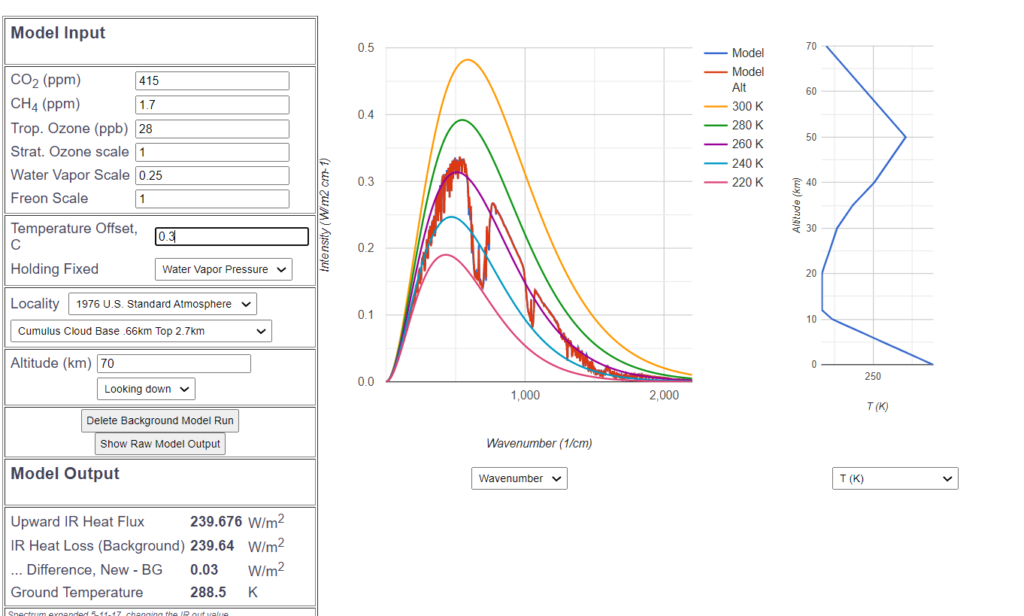
It is noticeable that the curves are almost identical and indistinguishable to the naked eye. The red curve almost completely obscures the blue one. Only at the calculated values in the left box you can see a slight difference. The appr. 1 $\frac{W}{m^2}$ lower radiation is compensated by a temperature increase of the earth surface of 0.3°. This average increase of 0.3° represents the hypothetical effective greenhouse effect from the beginning of industrialization until today, on the basis of the radiative transfer equations of the widely accepted MODTRAN model.

Now, what if we assume a doubling of $CO_2$ content from 280 ppm to 560 ppm? Again, the new curve is superimposed on the original blue curve.

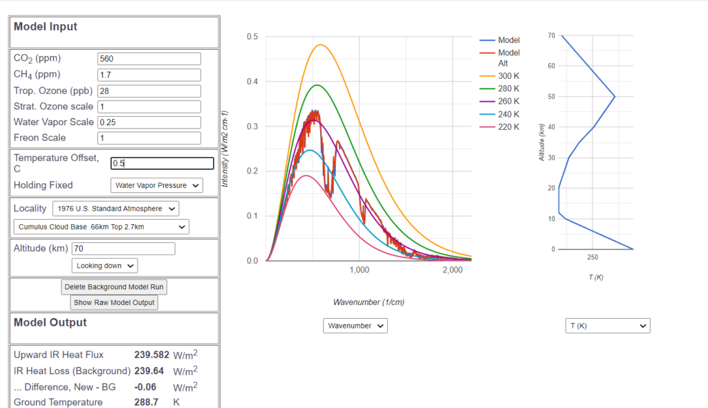
And again, to the naked eye, there is little difference – a few small blue peaks peek out at wavenumber 500, and the „$CO_2$ hole“ has become marginally wider, reducing the IR emission by $1.92\frac{W}{m^2}$. To compensate for the reduced infrared radiation due to this minimal greenhouse effect, the ground temperature is increased by a total of 0.5°C. Thus, the climate sensitivity according to the MODTRAN simulation is pretty much half a degree. A model to describe this measured sensitivity is described in this article.

In order to validate this result with data of the climate zone most relevant to a potential global warming, a corresponding scenario with a tropical atmosphere (27° C ground temperature, water vapor scale 0.5, Cumulus clouds) leads to a $CO_2$ sensitivity of 0.67° C in the tropical zone:

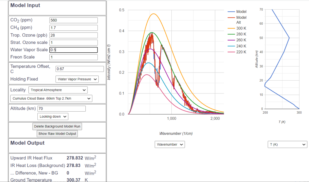
Therefore, there is no reason for any alarmism. These values ranging between 0.5 and 0.67 are far below the lowest assumptions of the Intergovernmental Panel on Climate Change.

Why does the IPCC reach different conclusions?

The natural question after these considerations is why the Intergovernmental Panel on Climate Change, which after all includes the best climate scientists, comes to such much more pessimistic conclusions?
A key problem here is that their climate models are extremely complex and claim to represent the full complexity of climate events. There are good reasons to believe that this is fundamentally impossible under current conditions, for example, because turbulent high-energy phenomena such as ocean currents or tropical storms are not adequately represented in these models. Similar models are used for weather forecasting, and these are already known to fail frequently for forecasts that extend beyond a few days.

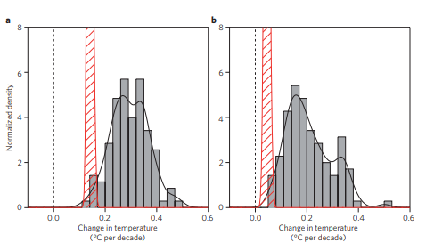
One important reason to doubt the validity of „global circulation models,“ or GCMs, is that they have consistently over-predicted past climate data in past forecasts.
On the left is the average temperature trend (red bar) 1993-2012 – 0.15°/10 years, on the right the same in the period 1998-2012 – 0.03°/10 years, and in addition the results of 110 different climate models. Almost all had estimated much higher temperatures.

Simulation of IPCC assumptions

With the MODTRAN simulation program, however, one can reproduce the thinking based on data published by authors close to the IPCC. This is done by first assuming an atmosphere entirely without water vapor and without the other greenhouse gases, and measuring the $CO_2$ sensitivity in such a hypothetical atmosphere.

With the MODTRAN simulation, this situation is achieved when everything in the standard atmosphere is set to 0 except for the $CO_2$ content, removing all clouds and water vapor.

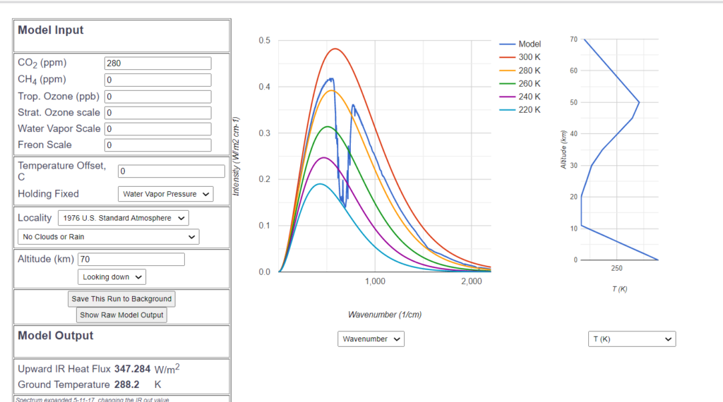
This, of course, raises the hypothetical radiation to an unrealistically high value of 347 $\frac{W}{m^2}$. Clearly, the only deviation from the „ideal curve“ is the well-known $CO_2$-hole.

When the $CO_2$ content is doubled and the ground temperature remains the same, the radiation now decreases by 3.77 $\frac{W}{m^2}$ due to the greenhouse effect.

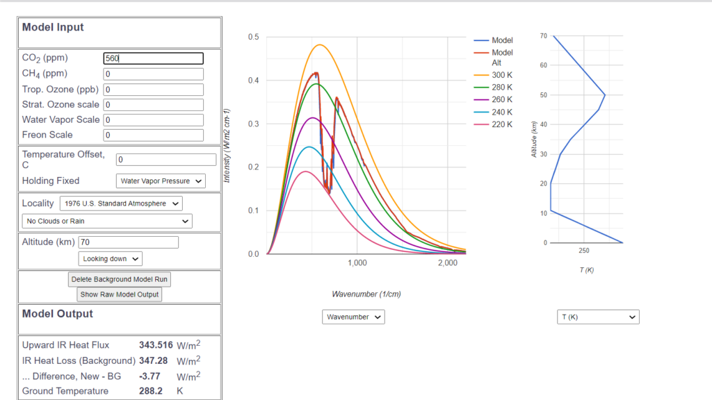
This is pretty much the value of $CO_2$ conditional „radiative forcing“ published by the Intergovernmental Panel on Climate Change. The reduced radiative forcing is compensated by temperature increase:

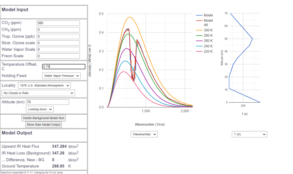
According to this, a temperature increase of 0.75° offsets the doubling of $CO_2$, which would be the sensitivity according to MODTRAN. However, many scientists arrive at an even higher sensitivity of about 1°.
But this sensitivity is called — in a way rightly — the „pure $CO_2$ sensitivity“ by scientists close to the IPCC, because it does not yet take into account the influence of water vapor. But since water vapor is an even more potent greenhouse gas, and more water vapor is produced by the $CO_2$-induced temperature increase, in this way of thinking the $CO_2$ sensitivity is thereby effectively doubled. Thus it is possible to arrive at a sensitivity of 2°, which can then be arbitrarily increased by other catastrophic scenarios such as hypothetical melting of polar ice. They completely disregard cumulus cloud formation, which would also be enhanced by increasing the water vapor content and which would lead to a reduction of the incident energy, i.e. to a strong negative feedback. At best, the cloud issue is used by arguing that the very high cirrus clouds may lead to an enhancement of the greenhouse effect.

Explanation of the discrepancy and conclusions

The large discrepancy between the IPCC published sensitivity of more than 2° C and the 0.5° C found by MODTRAN simulation requires a plausible explanation. Without entering the feedback discussion — which is of minor relevance in the case of very small sensitivitiy — here are two reasons for the deviations between the „pure“ $CO_2$-sensitivity of $3.77 \frac{W}{m^2}$ and the „Cloud-and-Water vapour“ sensitivity of $1.92 \frac{W}{m^2}$:

• As mentioned above the pure $CO_2$ sensitivity is based on an outgoing radiation of $347 \frac{W}{m^2}$, which is $1.1$%. Based on the real $240 \frac{W}{m^2}$, the same relative forcing of $1.1$% would result in $2.46 \frac{W}{m^2}$.
• The remaining difference between $2.46 \frac{W}{m^2}$ and $1.92 \frac{W}{m^2}$ can be explained with the fact that the presence of water vapour leads to a certain amount of competition in the emission of radiation in the uppor troposphere, with the result of a reduced forcing – some radiation which would be held back when no water vapour is present, is emitted through water vapour.
• One reason, why other investigations based on MODTRAN reach higher sensitivity, is the fact that some of them calculate the spectra from a height of 20 km instead of 70 km. This cuts off a considerable amount of the stratospheric $CO_2$ emissions, which have a — constant — cooling effect, thereby magnifying the warming effect of the remaining rest of $CO_2$.

Therefore, tearing apart $CO_2$, clouds, and water vapor when calculating $CO_2$ sensitivity is unwarranted. All factors need to be considered simultaneously, this leads to the low sensitivity of 0.5°.