Shares of anthropogenic and natural emissions in the increase in CO2 concentration

[latexpage]

The publication „Improvements and Extension of the Linear Carbon Sink Model“ shows that the global natural effective carbon sink depends on both the CO$_2$ concentration and the global (sea surface) temperature anomaly. A brief derivation of these relationships is provided below. In contrast to the cited publication, this investigation uses monthly deseasonalized CO₂ concentration data $C_i$, monthly global sea surface temperature data $T_i$, and monthly emission data $E_i$ from interpolated yearly emission data at consecutive months $i$ .

The conservation of mass or the continuity equation imply that the monthly concentration growth
$G_i=C_i-C_{i-1}$
necessarily results from the sum of anthropogenic emissions $E_i$ and natural emissions $N_i$ , reduced by the monthly absorptions $A_i$ :
\begin{equation}\label{eq:massconservation}
G_i = E_i + N_i – A_i
\end{equation}
By definition natural emissions here necessarily mean all CO₂ emissions except the anthropogenic emissions.
The measurable sink effect $S_i$ is the difference between anthropogenic emissions $E_i$ and the concentration growth $G_i$:
\begin{equation}\label{eq:sinkeffect}S_i = E_i – G_i\end{equation}

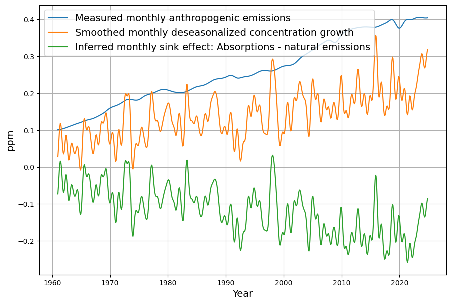
Figure 1: Emissions, concentration growth and sink effect(sink effect is plotted downwards).

It follows directly from equation 1 that the directly measurable sink effect $S_i$ includes not only absorptions by the oceans and plants, but implicitly also natural emissions:
$S_i = A_i – N_i$
Therefore, the sink effect is not identical to the sum of all absorptions, but only the proportion of absorptions that have not been compensated by natural emissions during the current month.

The work “ Improvements and Extension of the Linear Carbon Sink Model ” shows that the global sink effect $S_i$ is represented described by an extended model of CO$_2$ concentration and global sea surface temperature $T_i$:
\begin{equation}\label{eq:bilinearmodel} \hat{S}_i = a\cdot C_{i-1} +b\cdot T_{i-6} + c\end{equation}
As a matter of fact, the model fits best when there is a time lag of 6 months between temperature and sink effect.
The simple sink model described in the paper “Emissions and CO ₂ Concentration—An Evidence Based Approach ”, which depends only on the CO₂ oncentration, is used for comparison:
\begin{equation}\label{eq:linearmodel} \hat{S}_i = a’\cdot C_{i-1} + c’\end{equation}

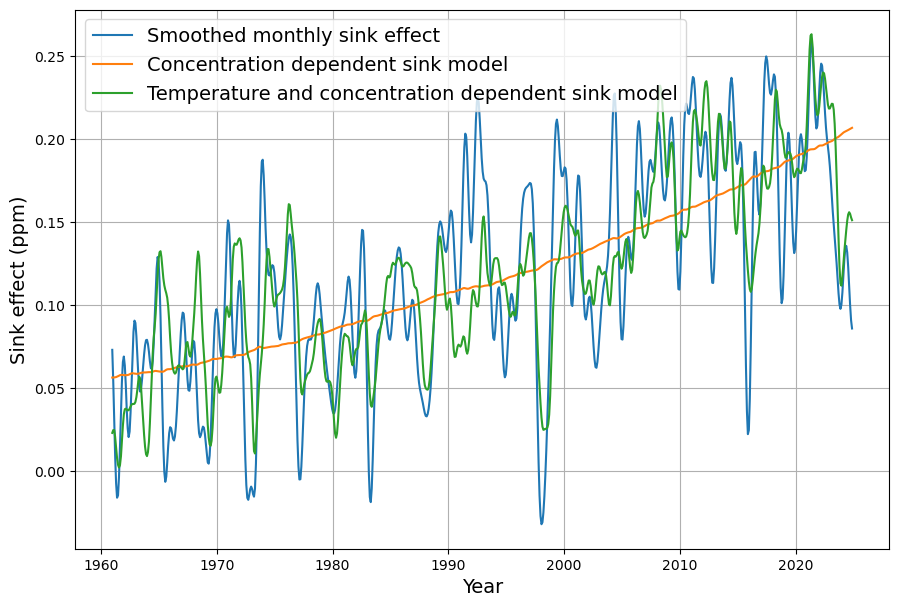
Figure 2 Modeling of the sink effect with a simple sink model (orange) and an extended sink model (green)

Figure 2 shows that the simple model reproduces the trend very well, but that the fluctuations can only be described by the extended model, i.e., by including dependence on the sea surface temperature. The parameters for the best fit of the extended model are $a=0,052$, $b=-4$ ppm/°C, $c=-16$ ppm.

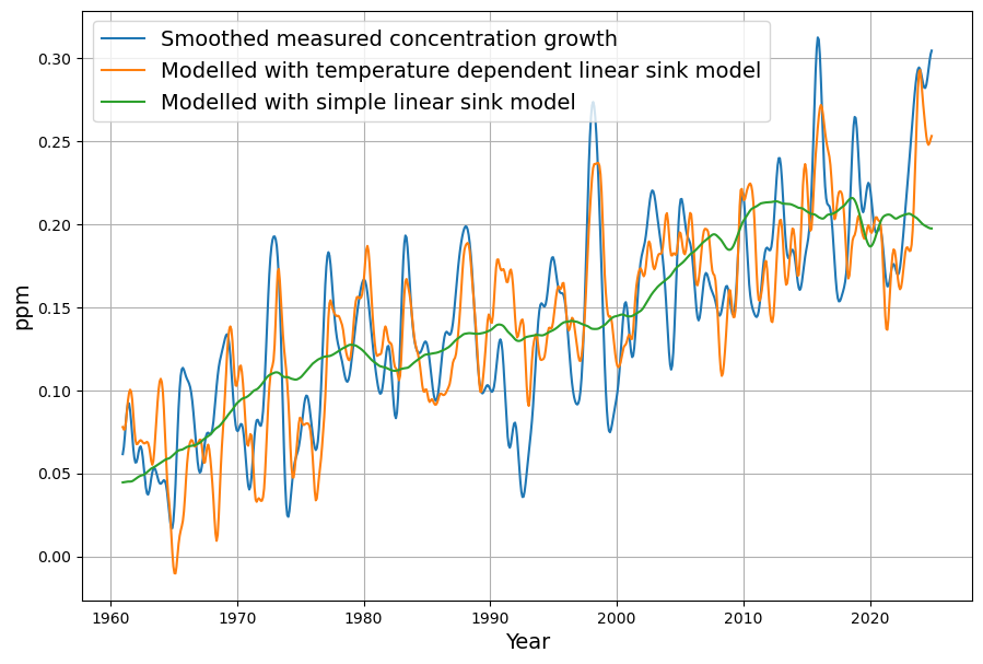
The increase in concentration can also be modeled using equations \ref{eq:sinkeffect}, \ref{eq:bilinearmodel}, and \ref{eq:linearmodel} respectively:
\begin{equation}\label{eq:g2model}\hat{G}_i = E_i – a\cdot C_{i-1} – b\cdot T_{i-1} – c\end{equation}
This is shown in Fig. 3. For comparison, the reconstruction with the simple sink model is shown here again (green curve).

Fig. 3: Measured concentration increase (blue), reconstructed with simple sink model (orange), reconstructed with extended sink model (green).

Reconstruction of concentration, differentiation of the influence of emissions and temperature

From the concentration growth, the course of the CO$_2$ concentration can be reconstructed using the initial CO$_2$ concentration , in this case the concentration in December 1958. According to equation 5, the concentration growth is controlled by the external state variables of anthropogenic emissions and temperature. Together with the determined parameter, the term results in the change in natural emissions due to the temperature anomaly . It is therefore interesting to first compare the magnitudes of both emission sources. The unit of measurement for emissions is GtC, which is calculated by multiplying the quantities otherwise measured in ppm by 2.123.

Figure 4 shows anthropogenic emissions since 1959 and natural emissions based on the sea surface temperature anomaly scale. Before 1975, temperatures and thus natural emissions, are predominantly negative. This is due to the arbitrary choice of the zero point of the anomaly temperature scale.

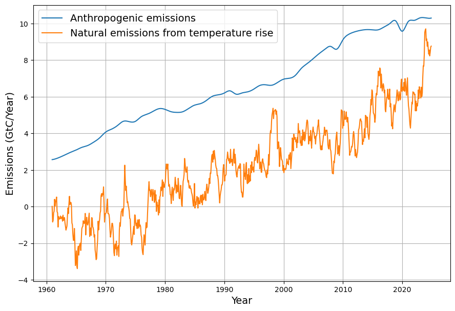
Figure 4: Anthropogenic emissions and temperature-induced natural emissions

It is noticeable that anthropogenic emissions are on average about 4 GtC larger than the natural emissions. Overall, natural emissions are numerically much larger, since the constant term of about 34 GtC (16 ppm \cdot 2.123 GtC/ppm) also represents natural emissions. According to equation 14 in Improvements and Extension of the Linear Carbon Sink Model, these constant natural emissions define the equilibrium concentration at the temperature anomaly 0°C; with current figures, this equilibrium concentration is 307 ppm. This is not the pre-industrial state, which has a temperature anomaly of -0.48°C. Fig. 5 shows three selected model scenarios. In addition to the actually measured concentration values, the reconstruction with the actual temperature and emission trends (orange) is shown. As expected, this remains very close to the measured data.

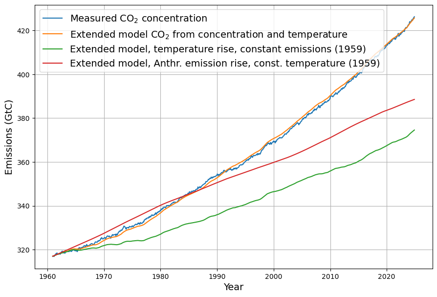
Figure 5: Measured concentration (blue), impact of three scenarios on the concentration. See text.

In addition, two further scenarios are presented:

Anthropogenic emissions remain at the 1959 level, and only the temperature continues to develop as we know it (green color). The CO₂ concentration increases to about 370 ppm.
The temperature remains at the 1959 level, but anthropogenic emissions continue to grow as usual. The concentration initially increases more steeply than if the temperature were also changing. This is because the temperature anomaly remains below zero until the mid-1970s. Only after 1983 does the resulting concentration remain below the reference value. Overall, anthropogenic emissions account for a larger share of the concentration increase than natural emissions, but in 2023, for example, the natural emissions share is very close to the anthropogenic emissions share.

It is also noticeable that the effects of both emission sources in terms of resulting concentration cannot simply be added together. The resulting concentration is lower than the sum of the concentrations of both emission components. This is due to the fact that absorption increases with increasing concentration. Both emission sources together have a smaller effect on the concentration than one would intuitively expect from their individual effects.

Discussion and Conclusions

The extended sink model allows us to consider the effects of anthropogenic emissions and temperature increases on CO₂ concentrations separately. This result contradicts those who believe that anthropogenic emissions fully explain the concentration changes since the beginning of industrialization. An insightful overview on this subject has been given by Ferdinand Engelbeen. His key argument in favour of the small contribution of natural emissions is that despite the initial yearly emission rate of 3..5 ppm/°C a saturation is reached, limiting the the equilibrium state concentration increase to 16 ppm/°C. This would prohibit an increase like the green curve in Figure 5, which rises by about 50 ppm for appr. 1°C temperature increase.
If we, however, restrict the concentration increase to 16 ppm (for the actual 1°C temperature increase), then due to the large absorption by 5.2% the anthropogenic emissions would not lead to the current 420 ppm but only to appr. 390 ppm. The evidence for the strong absorption of 5.2% is given by the fast decay of atmospheric $^{14}$C Data after the ban of bomb tests after 1963, which has a time constant of 17 years after Suess effect correction.
If we accept that the natural emissions of the ocean are restricted to a total of 16 ppm for a 1°C temperature rise, we need to consider the other possible source of natural emissions, the biological world. The decay of plants is a chemical process, following van’t Hoff’s rule, whereby the reaction velocity doubles for 10°C temperature rise. This means that for 1°C rise the increase of reaction velocity is appr. 7%. Therefore, we can expect a 7% rise of natural emissions based on the decay of biological material. With a total volume of 120 GtC per year of global primary production, which scales with both CO2 concentration and temperature, we can expect a rise of several GtC per year for natural emissions, even if the actual rise is smaller than the theoretical 7%.
The extended sink model also contradicts those who claim that, due to the large turnover of the natural carbon cycle, anthropogenic emissions play no role at all. It is actually trivial that anthropogenic emissions as a direct input must necessarily have an effect. The truth is that both factors have an influence of a similar order of magnitude, although anthropogenic emissions are slightly more predominant.