

IR re-emission – the traditional explanation
The communicated common understanding of the greenhouse effect depends very much on the re-emission hypothesis: Molecules of greenhouse gases such as  absorb infrared radiation, typically in the absorption band with the wavelength around
  , reaching an excited state. After some time the molecules return to the “ground state”, thereby emitting infrared radiation of the same wavelength isotropically. This is typically interpreted as radiating 50% upwards, and 50% downwards. Due to the assumption that all molecules do this, it is imagined that approximately half of the upwelling IR surface radiation is radiated back to the surface, resulting in “downwelling” IR. As this is additional heat reaching the surface, the surface is heated up. This is being called the “greenhouse effect”. Understandably the more there is in the atmosphere, the more it heats up.
With such a simple picture it is understandable that many claim that “the science is settled”.
Radiation is converted to thermal motion
A necessary condition for the behaviour described above to work, would be that the atmosphere was so thin that the probability for the decay of an excited -state is higher than the probability to collide with another gas molecule. In the real atmosphere, specifically the troposphere, the process is different. Let’s assume that molecules of the atmosphere are excited by infrared radiation (IR). This diagram shows,
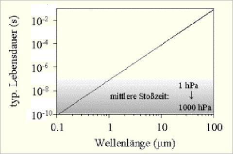
that the lifetime of an excited -molecule for wavelength  is appr.
  s. But the time between collisions with neighboring molecules is between
  s and
s and  s, depending on air pressure. Therefore the probability to transfer energy by collision is 10000-1000000 times larger than by re-emission. Additionally, the probablity to collide with a non- molecule is
  %.
%.
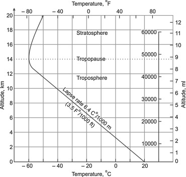
Collisions are described by thermodynamics. From gas law and energy conservation in the thermodynamic equlibrium this results in a state distribution described by the adiabatic barometric equations, essentially stating, that in an atmosphere subject to a gravitational field both density as well as temperature decrease with height above the surface. The temperature gradient is commonly called lapse rate. It is important to note that this temperature gradient is entirely caused by thermodynamics – it is the state of maximum entropy of a gas in a gravitational field, it has nothing to do with radiative forcing. For dry air the (dry adiabatic) lapse rate is  , only dependent on the gravitation constant and the specific heat, the moist adiabatic lapse rate includes the condensation heat of water vapor, and is in the range of
  , depending on the water vapor concentration.
Whereever heat is introduced into the atmosphere, it is forced to distribute thermodynamically across the whole atmosphere, with the equilibrium state of a temperature distribution according to the moisture dependent lapse rate. The so-called standard atmosphere has a lapse rate of  , which is approximately the measured global average lapse rate. This “thermodynamic forcing” is so overwhelmingly dominant (89%), that any other effects like radiative forcing are of minor significance within the troposphere. In the tropopause and above it is different. The atmosphere is so thin, that there is no thermodynamic equilibrium, and consequently the radiation effects dominate there.
Thermal motion is converted to radiation
Obviously the process also works in the other direction. A molecule may get excited by collisions and then radiates. But from the numbers above it is fairly clear, that direct re-emission plays a neglegible role in the interior of the troposphere: Any excited greenhouse gas molecule is overwhelmingly likely to distribute its additional energy to its neighbor molecules by collisions, the result is a local state of thermodynamic equilibrium. This is usually called “thermalisation” (interestingly Wikipedia does not mention atmospheric processes – honi soit qui mal y pense) . Therefore any selected volume sufficiently large to have a thermodynamic equilibrium can be regarded as an independent Planckian emitter of (infrared) radiation. So it is possible that a volume absorbing IR with is later emitting IR of another wavelength from water vapor (and vice versa). Thermodynamics permanently re-arranges the gas volume towards the local thermodynamic equilibrium. Any absorbed energy is locally quickly distributed across all neighboring molecules , some of which can radiate IR, and most others can’t. From such a volume you get a Planck emission spectrum involving all local greenhouse gases, not only .
Re-emission can therefore not be defined on a single molecule but emissions are independent of absorptions and are defined on a large enough volume to have a thermodynamic equilibrium.
Downwelling radiation and heat transport
According to Planck’s law a volume with higher temperature emits more radiation at all wavelengths. Volumes from higher altitudes emit less radiation because of temperature and densitiy gradients. Therefore upwelling radiation is always larger than downwelling radiation, with the important consequence that – under the condition of a lapse rate – there is no radiative heat transport from higher altitude to lower altitude. This is in accord with the 2nd law of thermodynamics, according to which heat can never flow spontaneously from a colder system to a warmer system.
Radiation at the boundary of the atmosphere
As soon as we are “close enough” to space, i.e. within 1 optical depth (which is wavelength dependent), then actual emission into space becomes possible, and takes place, because there are not enough suitable molecules above to absorb all radiation . Water vapor is by far the most relevant absorbing and emitting gas. Fig. 3 shows that there is a sharp drop of water vapor density at about 5 km altitude.

Radiative equilibrium at top of atmosphere
Whereas all energy-relevant interactions inside the atmosphere and between the atmosphere and the ground are based on convection(67%), evaporation/condensation(22%), and radiation(11%) – dominated by convection, the interaction with empty space is restricted to radiation. From the previous arguments it is clear, that relevant radiation is restricted to the “top of atmosphere”. To be precise, it is the range with less than 1 optical depth “distance” to empty space. This “distance scale” depends strongly on the wavelength of the infrared light.

From the emission spectrum of Outgoing Longwave Radiation (OLR) we can infer essentially 3 cases:
- At wavenumbers of
 there is the “atmospheric window”, where the (cloudless) atmosphere is nearly transparent to the infrared radiation – the optical depth spans the whole atmosphere, and the radiation temperature corresponds to the temperature of the earth’s surface of 280-310 K.
 - Between wavenumber
 there is the -Band. is homogeneously distributed in the atmosphere, with the radiation maximum in the stratosphere, corresponding to a rather low radiation temperature of about 220 K, a temperature amazingly stable w.r.t. both -concentration and surface temperature.
 - Overlapping with the band is the water vapor band from
 . From Fig. 3 follows that there is a sharp decline of water vapor concentration at 5 km height. Therefore the radiation temperature of the water vapor band is considerably higher than that of , appr. 250-280 K. Due to the fact that reaches higher altitudes due to homogeneous distribution, water vapor emissions within the -Band are absorbed by higher reaching molecules and are eventually emitted by at a higher altitude and mostly lower temperature (over Antarctica the emissions are at a higher temperature compared to the surface). This is the actual phenomenon that makes the greenhouse effect.
Lacking
- precise measurement data of these 3 emission components, measured locally at all latitudes,
- detailed knowlegde about cloud cover, which considerably changes the behaviour of the “atmospheric window”
we simplify the calculation by assuming an average “fixed” radiation height  of all 3 radiation components by demanding energy balance of averaged solar insolation and the validity of the Stefan-Boltzmann law at height h, with TOA incoming flux
  , global average albedo
  and the Stefan-Boltzmann constant
  and the wellknown result for the effective temperature:
![\[T_e = \sqrt[4]{\frac{S\cdot(1-\alpha)}{4\cdot \sigma} } = \sqrt[4]{\frac{1370 \cdot(1-0.3)}{4\cdot 5.67\cdot 10^{-8} } } K = 255 K\]](https://klima-fakten.net/wp-content/ql-cache/quicklatex.com-dd312495f2b2638b21818576313da4f1_l3.png "Rendered by QuickLaTeX.com")
Is global averaging legitimate?
I am aware that there are doubts about globally averaging the flux due to the nonlinear relation between flux and temperature as well as strongly changing flux and albedo with latitude (see also here, p. 18). I had these doubts myself, but considering all the other errors we make with such a simplified model, under the realistic condition of relatively small day/night temperature deviations due to heat storage ( within  ) the error of global averaging is small enough to be neglected (<1%), and the nonlinear SB equation can be expanded linearly around the global average flux
  and the global average temperature
  :
:
![\[\frac{\Delta T}{T_0} \approx \frac{1}{4}\cdot\frac{\Delta S}{S_0}\]](https://klima-fakten.net/wp-content/ql-cache/quicklatex.com-85b821f8bd95c66459f148c23222f44a_l3.png "Rendered by QuickLaTeX.com")
Interpretation of the effective Temperature
The key point here is that this effective temperature is not a surface temperature, but it is located somewhere in the atmosphere, “averaging” over the different levels of radiation of the contributing components. It is a fruitless undertaking to assume this to be a virtual surface temperature, leading to endless discussions about the underlying assumptions (what would be the “true” albedo, is liquid water heat storage “allowed”, is there no atmosphere or an atmosphere without greenhouse gases, etc. ). And, most important, only under the assumption of such a fictive surface temperature, the definition of which is rather arbitrary, “forcing” is required to “raise” the temperature to the level of the actual surface temperature.
The expected altitude of the equilibrium temperature  is easily computed from the assumed linear lapse rate (moist adiabatic lapse rate is not quite linear) and the actually measured average surface temperature
  :
:
![\[h=\frac{T_s-T_e}{\Gamma}=\frac{287-255}{6.4} km = 5 km\]](https://klima-fakten.net/wp-content/ql-cache/quicklatex.com-5ec5638162b3dc51483945012f87fd0b_l3.png "Rendered by QuickLaTeX.com")
It is important to note, that the lapse rate describes a state of an adiabatic thermodynamic equilibrium, i.e. the temperature difference between the surface and the the altitude
does not imply any energy imbalance in need of “forcing”. Regarding radiative processes (which contribute by 11% of the interaction in the troposphere) this thermodynamic equilibrium means that inbound radiation is equal to outbound radiation at each location, with thermodynamics governing the process. This equilibrium is, of course, only stable under the assumption of a constant in-flux at the surface or by direct atmospheric SW absorption which compensates the radiation losses at the top of atmosphere. Any changes such as day/night variation, seasonal or other weather variations obviously create energy fluxes, not to forget the permanent lateral flux due to latitudinal temperature gradients. The reactions to these are, however, always directed towards the entropy maximizing state of the optimal lapse rate.
In my understanding it is somehow misleading and the cause of misunderstandings to try to emulate the lapse rate equilibrium by means of virtual radiative fluxes. Nevertheless I do not deny the possibility to map the true thermodynamic behaviour into an “energy flux and budget” model, with (among other energy fluxes) 2 more or less equal radiative fluxes of different signs (downwelling and upwelling IR), both larger than the actual SW flux from the sun, as it is commonly done. The important constraint on these models must be that the partition temperatures are determined by the given lapse rate, so that the thermodynamic fundament constrains radiation. Only then the radiative model is consistent with the thermodynamic model. Undeniable fact is that only the – positive – difference  between upwelling and downwelling IR flux corresponds to an actual flow of heat:
![\[\Delta F=\epsilon\cdot (T_1^4 - T_2^4)\]](https://klima-fakten.net/wp-content/ql-cache/quicklatex.com-45a3789b51065f32d236c554b39c1bb7_l3.png "Rendered by QuickLaTeX.com")
All those who consider this approach to be “heretic”, may be reminded that James Hansen used the same logic and equations in the introduction of his famous 1984 paper.
The implications of this understanding regarding the -sensitivity are discussed on the page “Physics of the the Greenhouse effect” and regarding cloud and water vapor feedback on the page “Clouds and water vapor“.
One assumption that does bother me is that CO2 radiates only from a high altitude with a consequent temperature of about 220 K. If you look at the y-axis, it is in power i.e., “watts” (yours is milliwatts). The power radiated from a body depends on the surface area radiating. Basically how much material there is. It is not just one molecule, it is a number of them. With the assumption that a large percent of CO2 energy is dissipated through collisions, that means there is less, in fact far less number of CO2 molecules radiating. This by itself would reduce the power measured at the top of the atmosphere, that is, the “dip” you see in the spectrum around CO2. So, it could really be the volume of material causing the dip, and not the temperature. I have never seen any studies or papers that address this issue. They all assume that CO2 must be at a low temperature and simply ignore or don’t understand that reduced radiating volume could cause a similar reduction in power.
If you look carefully, the unit of the y-Axis is Watt/m^2 (irradiance or flux density), at the spectrum mW/(m^2*Sterad*cm^-1) (spectral radiance), which implies that it is normalized w.r.t the area, the 2D-angle (cone), and the wave number (see e.g. https://en.wikipedia.org/wiki/Irradiance). Therefore the spectrum does not depend on the area. The permanent absorption, dissipation, and emission leads to the effect that the atmosphere is opaque within the CO2-band. Maybe that is what you mean, too? Only the molecules within 1 “optical depth” can emit to space . Therefore it is also independent of the height of the column, only the molecules close enough to the top of atmosphere can emit to space. So it is normalized w.r.t. number of particles. The same applies to water vapor (at a lower height within the troposphere, say 5 km) . This is how greenhouse gases are defined. The “radiation temperature” depends on the temperature of the atmosphere from where the IR is emitted.
I think you misunderstand. It is normalized to area and wave number, but the power level is not. It is basically power per unit area. That is why the power curve moves up, more power.
The question is why less power at 15 um. There are a couple of reasons.
1. As you say, the atmosphere is opaque to 15 um which means that CO2 must be saturated, i.e. intercepting all 15 um radiation and passing it out the top.
2. There is only a small amount of 15 um radiation to be radiated. This can occur if most CO2 transfers energy to N2/O2.
I’ll finish later